The preseq Manual
Timothy Daley
Victoria Helus
March 21, 2014
Andrew Smith
Contents
1
Quick Start
2
2
Installation
3
3
Using preseq
4
4
File Format
5
5
Detailed usage
6
6
lc extrap Examples
8
7
preseq Application Examples
11
8
FAQ
15
1
1
Quick Start
The preseq package is aimed at predicting the yield of distinct reads from a genomic library from an initial
sequencing experiment. The estimates can then be used to examine the utility of further sequencing, optimize the sequencing depth, or to screen multiple libraries to avoid low complexity samples.
The three main programs are c curve, lc extrap, and gc extrap. c curve samples reads without
replacement from the given mapped sequenced read file or duplicate count file to estimate the yield of the
experiment and the subsampled experiments. These estimates are used construct the complexity curve of the
experiment. lc extrap uses rational function approximations of Good & Toulmin’s [3] non-parametric
empirical Bayes estimator to predict the yield of future experiments, in essence looking into the future for
hypothetical experiments. lc extrap is used to predict the yield and then c curve can be used to check
the yield from the larger experiment.
gc extrap uses rational function approximations to Good & Toulmin’s estimator to predict the genomic coverage, i.e. the number of bases covered at least once, from deeper sequencing in a single cell or
low input sequencing experiment based on the observed coverage counts. The option is available to predict
the coverage based on binned coverage counts to speed up the estimates. gc extrap requires mapped read
or bed format input, so the tool bam2mr is provided to convert bam format read to mapped read format.
2
2
Installation
Download
preseq is available at http://smithlab.cmb.usc.edu/software/.
System Requirements
preseq runs on Unix-type system with GNU Scientific Library (GSL), available at
http://www.gnu.org/software/gsl/. If the input file is in BAM format, SAMTools is required,
available at http://samtools.sourceforge.net/. If the input is a text file of counts in a single
column or is in BED format, SAMTools is not required. It has been tested on Linux and Mac OS-X.
Installation
Download the source code and decompress it with
$ tar -jxvf preseq.tar.bz2
Enter the preseq/ directory and run
$ make all
The input file may possibly be in BAM format. If the root directory of SAMTools is $SAMTools, instead
run
$ make all SAMTOOLS_DIR=$SAMTools
Output after typing this command should include the flag -DHAVE SAMTOOLS if the linking is successful.
If compiled successfully, the executable file is available in preseq/.
If a BAM file is used as input without first having run $ make all SAMTOOLS DIR=/loc/of/SAMTools,
then the following error will occur: terminate called after throwing an instance of
’std::string’.
3
3
Using preseq
Basic usage
To generate the complexity plot of a genomic library from a read file in BED or BAM format or a duplicate
count file, use the function c curve. Use -o to specify the output name.
$ ./preseq c_curve -o complexity_output.txt input.bed
To estimate the future yield of a genomic library using an initial experiment in BED format, use the
function lc extrap. The required options are -o to specify the output of the yield estimates and the
input file, which is either a BED file sorted by chromosome, start position, end position, and strand or a
BAM file sorted with the SAMTools sort function. Additional options are available and are detailed below.
$ ./preseq lc_extrap -o future_yield.txt input.bed
For a low input sequencing experiment the genomic coverage is highly variable and uncertain function of
sequencing depth. Some regions may be missing due to locus dropout or preferentially amplified during
MDA (multiple displacement amplification). gc extrap allows the level genomic coverage from deep
sequencing to be predicted based on an initial sample. The input file format need to be a mapped read
(MR) or BED, sorted by chromosome, start position, and end position. Additional options are available and
are detailed below.
$ ./preseq gc_extrap -o future_coverage.txt input.mr
4
4
File Format
Sorted read files in BED or BAM format
Input files are sorted mapped read files in BED or BAM format, or a text file consisting of one column
giving the observed read counts. The programs require that BED files are sorted by chromosome, start
position, end position, and strand. This can be achieved by using the command line function sort as follows:
sort -k 1,1 -k 2,2n -k 3,3n -k 6,6 input.bed > input.sort.bed
BAM format read files should be sorted by chromosome and start position. This can be done with the
SAMTools sort function. If the input is in BAM format, then the flag -B must be included.
If the input is paired end, the option -P can be set. In this case concordantly mapped reads and
disconcordantly mapped fragments are counted. This means that both ends of a disconcordantly mapped
read will each be counted separately. If a large number of reads are disconcordant, then the default single
end should be used. In this case only the mapping location of the first mate is used as the unique molecular
identifier [4].
Text files of observed read counts
For more general applications preseq allows the input to be a text file of observed read counts, one count
per line. To specify this input, the option -V must be set.
Such a text file can typically be constructed by command line arguments. Take for example an unmapped
sequencing experiment in FASTQ format. To predict the complexity, the unique molecular identifier needs
to use only the observed sequence. For instance, a unique molecular identifier used may be the first 20
bases in the observed sequence. A command line argument to construct the counts would then be
awk ’{ if (NR%4==2) print substr($0,1,20); }’ input.fastq | sort | uniq -c
| awk ’{ print $1 }’ > counts.txt
More complicated unique molecular identifiers can be used, such as mapping position plus a random
barcode, but are too complicated to detail in this manual. For questions with such usage, please contact us
at [email protected]
Mapped read format for gc extrap
gc extrap does not allow for input files to be in BAM format. We have found that some mappers give
inconsistent SAM flags for paired end reads, preventing proper merging of reads in the proper order. We
provide the tool bam2mr to convert SAM or BAM format files to MR format. The MR or BED format file
needs to be sorted by chromosome, start, and end position before input into gc extrap.
5
5
Detailed usage
c curve
c curve is used to compute the expected complexity curve of a mapped read file by subsampling smaller
experiments without replacement and counting the distinct reads. Output is a text file with two columns.
The first gives the total number of reads and the second the corresponding number of distinct reads.
-o, -output
Name of output file. Default prints to screen
-s, -step
The step size for samples. Default is 1 million reads
-v -verbose
Prints more information
-B, -bam
Input file is in BAM format
-P, -pe
Input is a paired end read file
-H, -hist
Input is a text file of the observed histogram
-V, -vals
Input is a text file of read counts
lc extrap
lc extrap is used to generate the expected yield for theoretical larger experiments and bounds on the
number of distinct reads in the library and the associated confidence intervals, which is computed by
bootstrapping the observed duplicate counts histogram. Output is a text file with four columns. The first is
the total number of reads, second gives the corresponding average expected number of distinct reads, and
the third and fourth give the lower and upper limits of the confidence interval. Specifying verbose will print
out the counts histogram of the input file.
-o, -output
Name of output file. Default prints to screen
-e, -extrap
Max extrapolation. Default is 1 × 1010
-s, -step
The step size for samples. Default is 1 million reads
-n, -bootstraps
The number of bootstraps. Default is 100
-c, -cval
Level for confidence intervals. Default is 0.95
-d, -dupl level
Fraction of duplicates to predict. Default is 0.5
-x, -terms
Max number of terms for extrapolation. Default is 100
-v -verbose
Prints more information
-B, -bam
Input file is in BAM format
-P, -pe
Input is a paired end read file
-H, -hist
Input is a text file of the observed histogram
6
-V, -vals
Input is a text file of read counts
-Q, -quick
Quick mode, option to estimate yield without bootstrapping for
confidence intervals
gc extrap
For single cell or low input sequencing experiments gc extrap is used to extrapolate the expected
number of bases covered at least once for theoretical larger experiments. Output is a text file with four
columns. The first is the total number of sequenced and mapped bases, second gives the corresponding
expected number of distinct bases covered, and the third and fourth give the lower and upper limits of the
confidence interval. Specifying verbose will print out the coverage counts histogram of the input file.
-o, -output
Name of output file. Default prints to screen
-w, -max width
max fragment length, set equal to read length for single end reads
-b, -bin size
bin size. Default is 10
-e, -extrap
Maximum extrapolation in base pairs. Default is 1 × 1012
-s, -step
The step size in bases between extrapolation points. Default is 100
million base pairs
-n, -bootstraps
The number of bootstraps. Default is 100
-c, -cval
Level for confidence intervals. Default is 0.95
-x, -terms
Max number of terms for extrapolation. Default is 100
-v -verbose
Prints more information
-D, -bed
Input file is in BED format without sequence information
-Q, -quick
Quick mode, option to estimate genomic coverage without
bootstrapping for confidence intervals
7
6
lc extrap Examples
Usage and output of c curve is similar, so the following examples are of lc extrap and its different
options.
Using a sorted read file in BED (or BAM with the -B flag) format as input
$ ./preseq lc_extrap -o future_yield.txt input.bed
TOTAL READS
0
1000000.0
2000000.0
3000000.0
4000000.0
.
.
.
.
9999000000.0
EXPECTED DISTINCT
0
955978.6
1897632.0
2829410.5
3751924.0
.
.
.
.
185394069.4
LOGNORMAL LOWER 95%CI
0
953946.4
1892888.4
2819146.4
3732334.5
.
.
.
.
76262245.8
LOGNORMAL UPPER 95%CI
0
958015.1
1902387.5
2839712.0
3771616.2
.
.
.
.
450694319.0
This example uses a sorted read file in BED format from an initial experiment generated from single sperm
cells. As noted above, the default step size between yield estimates is 1 million, the default confidence
interval level is 95%, and the default extrapolation length is 10 billion.
Using a sorted read file in BED format as input, including the verbose option
$ ./preseq lc_extrap -o future_yield.txt input.bed -v
As lc extrap is running, information will print to screen that gives a read counts histogram of the input
file which truncates after the first bin value that has zero observations. Included here is the first 10 lines of
what would be observed:
TOTAL READS
DISTINCT READS
DISTINCT COUNTS
MAX COUNT
COUNTS OF 1
MAX TERMS
OBSERVED COUNTS
1
511413
2
2202
3
597
.
.
= 536855
= 516200
= 48
= 269
= 511413
= 100
(270)
8
Using a sorted read file in BED format as input, with options
$ ./preseq lc_extrap -e 15000000 -s 500000 -b 90 -c .90 -o future_yield.txt input.bed
TOTAL READS
0
500000.0
1000000.0
1500000.0
2000000.0
.
.
.
.
14500000.0
EXPECTED DISTINCT
0
481098.5
956070.6
1428183.4
1897886.0
.
.
.
.
12932529.0
LOGNORMAL LOWER 90%CI
0
480329.1
954493.7
1425461.7
1892501.7
.
.
.
.
12056525.8
LOGNORMAL UPPER 90%CI
0
481869.1
957650.2
1430910.2
1903285.7
.
.
.
.
13872180.9
Notice the slight changes, with the step sizes of the extrapolation now at 500,000 as specified, and the
maximum extrapolations ending at 15,000,000. The confidence intervals are now at a level of 90%.
Using a histogram or read counts as input
lc extrap allows the input file to be an observed histogram. An example of the format of this histogram
is as followed:
1
2
3
4
5
6
7
8
9
10
1.68166e+07
4.55019e+06
1.93787e+06
1.07257e+06
708034
513134
384077
282560
206108
146334
The following command will give output of the same format as the above examples.
$./preseq lc_extrap -o future_yield.txt -H histogram.txt
Similarly, both lc extrap and c curve allow the option to input read counts (text file should contain
ONLY the observed counts in a single column). For example, if a dataset had the following counts
histogram:
1
2
3
4
3
1
9
Then, the corresponding input file of just read counts could be as such:
1
2
1
1
3
2
2
1
Command should be run with the -V flag (not to be confused with -v for verbose mode):
$./preseq lc_extrap -o future_yield.txt -V counts.txt
10
7
preseq Application Examples
Screening multiple libraries
This section provides a more detailed example using data from different experiments to illustrate how
preseq might be applied. Because it is important to avoid spending time on low complexity samples, it is
important to decide after observing an initial experiment whether or not it is beneficial to continue with
sequencing. The data in this example comes from a study (accession number SRA061610) using single cell
sperm cells amplified by Multiple Annealing and Looping Based Amplification Cycles (MALBAC) [5] and
focuses on three libraries coming from different experiments from the study (SRX205369, SRX205370,
SRX205372).
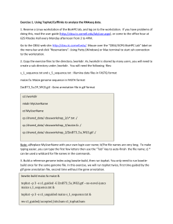
These libraries help show what would be considered a relatively poor library and a relatively good library,
as well as compare the complexity curves obtained from running c curve and lc extrap, to show how
lc extrap would help in the decision to sequence further. The black diagonal line represents an ideal
library, in which every read is a distinct read (though this cannot be achieved in reality). The full
experiments were down sampled at 5% to obtain a mock initial experiment of the libraries, as shown here,
where we have the complexity curves of the initial experiments generated by c curve:
6
distinct reads (M)
5
4
3
2
1
0
0
1
SRX205372
Lu et al. Science 2012
2
3
4
total reads (M)
SRX205369
Figure 1: Initial observed complexities
11
5
6
SRX205370
With such a relatively small amount of reads sequenced, it is hard in the first stages of a study to guess at
whether it is not worth sequencing a library further, as all three libraries seem to be relatively good.
This is a comparison of the full experiment complexity curves and the extrapolated complexity curves
created using information from the initial experiments above as input. The dashed lines indicate the
complexity curves predicted by lc extrap, and the solid lines are the expected complexity curves of the
full experiments, obtained using c curve. Note that the dashed curves follow the solid curves very
closely, only differing slightly towards the end, meaning lc extrap gives a good predicted yield curve.
Using this, it is clear that if the initial experiments were the only available data and lc extrap was run,
SRX205372 would likely be discarded, as it is a poor library, and SRX205369 and SRX205370 would
probably be used for further sequencing, as their complexity curves indicate that sequencing more would
yield enough information to justify the costs. If the researcher were to only want to sequence one library
deep, then SRX205370 would be an obvious choice.
100
distinct reads (M)
80
60
40
20
0
0
20
40
60
total reads (M)
SRX205372
SRX205369
observed
predicted
observed
predicted
80
SRX205370
observed
predicted
Figure 2: Estimated versus observed library complexities.
12
100
Saturation of reads and junctions for RNA sequencing experiments
A recent paper from the Rinn lab [6] developed a targeted capture RNA sequencing protocol to deeply
investigate chosen portions of the transcriptome. A comparison of the results from a standard RNA
sequencing experiment (RNA-seq; SRA accession SRX061769) and a targeted capture RNA sequencing
experiment (Capture-seq; SRA accession SRX061768) reveals a startling amount of transcriptional
complexity missed by standard RNA sequencing in the targeted regions. A large number of rare
transcriptional events such as alternative splices, alternative isoforms, and long non-coding RNAs were
newly identified with the targeted sequencing.
A current vigorous debate exists on whether these rare events are truly transcriptional events or are merely
due to sequencing or transcriptional noise (see [7] and [2]). We do not seek to address these issues, but
merely to comment on the true complexity of rare transcriptional events in sequencing libraries identified
by current protocols.
We took the two Illumina sequencing libraries from [6] and mapped them according to the protocol given.
We downsampled 10% of the library and compared the estimated library complexities (single end) with the
observed library complexity for both libraries. We also took the junction information contained in the file
junctions.bed in the Tophat output folder to estimate the junction complexity. Since the 5th column
(excluding the first line) is the number of times each distinct junction is observed, we can simply cut out
these values as input for lc extrap or c curve with the flag -V. A simple command line example
follows.
sed ’1d’ tophat/junctions.bed | cut -f 5 > junction_vals.txt
./preseq lc_extrap -V junction_vals.txt -o junction_vals_extrap.txt
The output TOTAL READS column will be in terms of the number of total junctions (not reads), so scaling
by the average number of junctions per read will give the appropriate scale for plotting on the x-axis.
200
distinct junctions (thousands)
distinct reads (millions)
20
15
10
5
0
150
100
50
0
0
10
20
30
40
50
60
0
total reads (millions)
10
20
30
40
50
60
total reads (millions)
RNA-seq
observed
Capture-seq
observed
estimated
estimated
Figure 3: A comparison of complexities of standard RNA-seq and targeted capture RNA-seq. Estimated
complexities for both cases were estimated using 10% of the data.
13
We see from the estimated library that the RNA-seq library is far from saturated, while it appears that the
Capture-seq library may be close. On the other hand, the junction complexity of both libraries indicates
that the full scope of juctions identified by Tophat is far from saturated in both libraries. This indicates that
large number of rare junctions still remain to be identified in the libraries.
14
8
FAQ
1. Q — When compiling the preseq binary, I receive the error
fatal error: gsl/gsl cdf.h: No such file or directory
A. — The default location of the GSL library will be in ’/usr/local/include/gsl’. Open
the Makefile and append ”-I /usr/local/include” after CXX = g++. You may be
receiving this error because the GSL library is not installed on the default search paths of your
compiler, and you will need to specify the location.
2. Q — When compiling the preseq binary, I receive the error
Undefined symbols for architecture x86 64:
" packInt16", referenced from:
deflate block in bgzf.o
" packInt32", referenced from:
deflate block in bgzf.o
" unpackInt16", referenced from:
bgzf read block in bgzf.o
check header in bgzf.o
A. — Go to the SAMTools directory and open the file bgzf.c. Find the functions packInt16,
unpackInt16, and packInt32. Comment out the ”inline” before each function name.
3. Q — I compile the preseq binary but receive the error
terminate called after throwing an instance of ’std::string’
A. — This error is typically called because either the flag -B was not included to specify bam input
or because the linking to SAMTools was not included when compiling preseq. To ensure that the
linking was done properly, check for the flag -DHAVE SAMTOOLS.
4. Q — When running lc extrap, I receive the error
ERROR: too many iterations, poor sample
A. — Most commonly this is due to the presence of defects in the approximation which cause the
estimates to be unstable. Setting the step size larger (with the flag -s) will help to avoid the
defects. The default step size is 1M reads or 0.05% of the input sample size rounded up to the
nearest million, whichever is larger. A consequence of this action will be a reduction in the
observed smoothness of the curve.
5. Q — When running lc extrap, I receive the error
sample not sufficiently deep or duplicates removed
A. — There may be two causes for this, either duplicates have been removed and every observed
read is distinct or there is not sufficient variation in the library for lc extrap to run.
15
The information required by lc extrap is essentially the number of times each distinct read was
observed, which we call the duplicate counts. Without sufficient variation in the duplicate counts
we cannot extrapolate the complexity of the library. We have set the minimum required max
duplicate count (the largest number of times any read has been observed) to 4. If the input library
does not satisfy this, then either a parametric model such as a Poisson or Negative Binomial may
be appropriate or deeper sequencing may be required.
6. Q — When running lc extrap, I receive the error
Library expected to saturate in doubling of size, unable to extrapolate
A. — A simple two-fold extrapolation using the Good-Toulmin power series, which is within the
radius of convergence and therefore rational function approximation is not needed, is performed to
ensure that the sample is not overly saturated. If the Good-Toulmin formula is negative, this
indicates that the library will likely completely saturate by doubling the experiment size and so
extrapolation is not needed. Often this will occur if the number of reads observed twice (n2 ) is
greater than the number of reads observed once (n1 ). In this case one can use simple estimators
like Chao’s [1] (n21 /2n2 ) or Zelterman’s [8] (1/(exp(2n2 /n1 ) − 1)) can be used to estimate the
number of remaining in the library.
If none of these solutions worked, please email us at [email protected] and please include the standard
output from running preseq in verbose mode (specifically the duplicate counts histogram) so that we can
look into the problem and rectify problems in future versions. Also, feel free to email us with any other
questions or concerns. The preseq software is still under development so we would appreciate any advice,
comments, or notification of any possible bugs. Thanks!
16
References
[1] Anne Chao. Estimating the population size for capture-recapture data with unequal catchability.
Biometrics, pages 783–791, 1987.
[2] Michael B Clark, Paulo P Amaral, Felix J Schlesinger, Marcel E Dinger, Ryan J Taft, John L Rinn,
Chris P Ponting, Peter F Stadler, Kevin V Morris, Antonin Morillon, et al. The reality of pervasive
transcription. PLoS biology, 9(7):e1000625, 2011.
[3] I. J. Good and G. H. Toulmin. The number of new species, and the increase in population coverage,
when a sample is increased. Biometrika, 43:45–63, 1956.
[4] T. Kivioja, A. V¨ah¨arautio, K. Karlsson, M. Bonke, M. Enge, S. Linnarsson, and J. Taipale. Counting
absolute numbers of molecules using unique molecular identifiers. Nature Methods, 9:72–74, 2012.
[5] Sijia Lu, Chenghang Zong, Wei Fan, Mingyu Yang, Jinsen Li, Alec R Chapman, Ping Zhu, Xuesong
Hu, Liya Xu, Liying Yan, et al. Probing meiotic recombination and aneuploidy of single sperm cells by
whole-genome sequencing. Science, 338(6114):1627–1630, 2012.
[6] T.R. Mercer, D.J. Gerhardt, M.E. Dinger, J. Crawford, C. Trapnell, J.A. Jeddeloh, J.S. Mattick, and J.L.
Rinn. Targeted RNA sequencing reveals the deep complexity of the human transcriptome. Nature
Biotechnology, 30(1):99–104, 2011.
[7] Harm van Bakel, Corey Nislow, Benjamin J Blencowe, and Timothy R Hughes. Most dark matter
transcripts are associated with known genes. PLoS biology, 8(5):e1000371, 2010.
[8] Daniel Zelterman. Robust estimation in truncated discrete distributions with application to
capture-recapture experiments. Journal of statistical planning and inference, 18(2):225–237, 1988.
17