
playoff - Tusseklubben
Workshop on Farm Animal and Food Quality Imaging 2013 Espoo, Finland, June 17, 2013 Proceedings DTU Compute-‐Technical Report-‐2013-‐12 Organizers: Assistant Professor Line Clemmensen, Technical University of Denmark Professor Rasmus Larsen, Technical University of Denmark Professor Bjarne Ersbøll, Technical University of Denmark Professor Chris Glasbey, Biomathematics & Statistics Scotland List of content Author Title Pages Milan Sonka Just Enough Interac/on Paradigm and Graph Algorithmic Techniques: Transla/on to Farm Animal and Food Quality Image Analysis 5-‐6 Anton Bardera , Jørgen Kongsro & A new segmenta/on framework for in vivo internal Imma Boada organs removal of CT scans of pigs 7-‐12 Jørgen Kongsro & Eli Gjerlaug-‐ Enger How to measure meat quality in vivo? An example using 13-‐14 computed tomography (CT) for measuring intramuscular fat (IMF) in live breeding pigs. Michael Judas & Anja Petzet Sta/s/cal dissec/on -‐ for which /ssues does PLS regression work? 15-‐20 Mathieu Monziols, Julien Faixo, Elias Zahlan & Gerard Daumas So?ware for automa/c treatment of large biomedical images databases 21-‐26 Andy Bulpi@ Building models from Biomedical Images: From cell structure to organ func/on 27-‐28 Claus Borggaard Mul/spectral vision for on-‐line inspec/on of meat 29-‐32 Murat Kulahci Mul/variate Sta/s/cal Process Control 33-‐34 Ruta Gronskyte, Murat Kulahci & Monitoring mo/on of pigs in thermal videos Line K. H. Clemmensen 35-‐40 Author Title Pages Hildur EinarsdoQr, Mikkel S. Contextual mul/variate segmenta/on of meat Nielsen, Bjarne K. Ersbøll, products from gra/n-‐based mul/modal x-‐ray Rasmus Larsen, MarSn Bech, tomography Franz Pfeiffer, Lars B. Christensen & Robert Feidenhans’l 41-‐46 Camilla H. Trinderup, Anders L. U/liza/on of mul/spectral images for meat color Dahl, Jens M. Carstensen & Knut measurements Conradsen 47-‐52 Anders B. L. Larsen, Marchen S. An explora/ve study on pork loin recogni/on Hviid, Rasmus Larsen & Anders L. Dahl 53-‐58 Flemming Møller Segmenta/on and color quan/fica/on of salamis -‐ 59-‐60 by combining supervised models Jannic B. Nielsen & Anders B. L. Larsen Online Mul/-‐Spectral Meat Inspec/on 61 Workshop on Farm Animal and Food Quality Imaging June 17th, 2013 Just Enough Interaction Paradigm and Graph Algorithmic Techniques: Translation to Farm Animal and Food Quality Image Analysis Milan Sonka ([email protected]) The Iowa Institute for Biomedical Imaging The University of Iowa Abstract. Accurate and reliable image analysis is of paramount importance in medical image analysis. With a widespread use of 3D/4D imaging modalities like MR, MDCT, ultrasound, or OCT in routine clinical practice, physicians are faced with ever-increasing amounts of image data to analyze and quantitative outcomes of such analyses are increasingly important. Yet, daily interpretation of clinical images is still typically performed visually and qualitatively, with quantitative analysis being an exception rather than the norm. Since performing organ/object segmentations in 3D or 4D is infeasible for a human observer in clinical setting due to the time constraints, quantitative and highly automated analysis methods must be developed. For practical acceptance, the method must be robust in clinical-quality images and must offer close-to 100% success rate – possibly using minimal expert-user guidance following the Just Enough Interaction (JEI) paradigm. Our method for simultaneous segmentation of multiple interacting surfaces belonging to multiple interacting objects will be presented. The reported method is part of the family of graph-based image segmentation methods dubbed LOGISMOS for Layered Optimal Graph Image Segmentation of multiple Objects and Surfaces. This family of methods guarantees solution optimality with directly applicability to n-D problems. To solve the issue of close-to 100% performance in clinical data, the JEI paradigm is inherently tied to the LOGISMOS approach and allows highly efficient minimal (just-enough) user interaction to refine the automated segmentation. Practically acceptable results are obtained in each and every analyzed scan with no or only small increase in human analyst effort. The performance of the minimally-guided JEI method will be demonstrated on pulmonary CT and coronary IVUS image data and translation to farm animal and food quality imaging will be discussed. 1 Workshop on Farm Animal and Food Quality Imaging June 17th, 2013 2 Workshop on Farm Animal and Food Quality Imaging June 17th, 2013 A New Segmentation Framework for in vivo Internal Organs Removal of CT Scans of Pigs Anton Bardera1 , Jørgen Kongsro2 , and Imma Boada1 1 GILab, University of Girona 2 Norsvin, Norway Abstract. The grading of farmed animal carcasses depends on the content of lean meat, fat and bone. Current imaging technologies are able to detect and represent carcass composition in images. To extract information from these images, specialized image processing techniques are required. In this paper, we propose a new segmentation method to accurately separate lean meat, fat and bone from a set of images from Computed Tomography scans. The main challenge is the detection of the internal organs, such as the lungs, the liver, and the kidneys, which are not considered in the manual dissection. The proposed approach has been tested on real data sets, and compared with manual dissection. The obtained results prove the high correlation between the virtual and manual dissection. 1 Introduction Measuring the composition of a farm animal is of great importance since this is the basis of the entire payment and breeding system of animals. Grading and classification of farmed animal carcasses is based on the content of lean meat, fat and bone. The producers are paid by the lean meat content relative to the other body tissues (lean meat percentage or LMP). Predicting LMP is done by various methods based on type of animal (specie), sex, age and available technology. The reference method for prediction of LMP is dissection. Since the invention of X-ray, ultrasound, computed tomography (CT) and magnetic resonance imaging (MRI), imaging has been applied to estimate and predict the body composition of farmed animals. Imaging technology provides non-invasive, and more objective and accurate estimates of body composition compared to more subjective and invasive methods like visual and probe grading. During the last decade, CT and MRI have shown that they can be used as an alternative to dissection, replacing the current subjective reference method, usually based on dissection. This may lead towards a greater harmonization between countries applying the same grading and classification system for farmed animal carcasses. Imaging methods will therefore play a decisive role, both for predicting and estimating body composition or LMP, and as a reference method. For breeders, farmers, producers, meat industry and consumers, accuracy and objectivity is very important to get the best possible quality and value for the money, from farm to fork. 3 Workshop on Farm Animal and Food Quality Imaging June 17th, 2013 Medical image advances, as well as, the advances in the area of computer science and video processing have created new ways to monitor quality in the food industry. Studies based on tomographic slice data obtained from CT or MRI have become a common practice in the meat industry. In this new context, the development of software platforms integrating image processing and visualization techniques able to process meat image data have become fundamental. In this paper, we focus on the automatic quantification of lean meat, fat and bone from CT images. We propose a new image processing framework based on several state-of-the-art segmentation techniques to exclude the parts of the pig that are not considered in the manual dissection, i.e. internal organs, and to correctly classify the other tissues. The proposed approach has been tested on different data sets and compared with manual dissection. The obtained results show that our method highly correlates with manual dissection. This paper is organized as follows. In Section 2, we review previous work related to the proposed approach. In Section 3, we introduce a new processing pipeline to automatically detect the lean meat percentage. In Section 4, we analyze the performance of the proposed approach on different input data sets. Finally, in Section 5, we present the conclusions and future research. 2 Previous Work Estimating body composition by of farmed animals requires a lot of sampled images. In example, modern CT scanners can generate a large number (1000+ images) of slices of a whole body to construct a body volume. The interpretations of these large numbers of images need a lot of time and energy [1]. A computer-aided system or an algorithm which handles these images automatically will speed up the process and reduce human errors. Such a system requires computer intensive methods and programming. A detailed flow of process must be designed, i.e. from removal of internal organs to produce a carcass from a live animal to classification of different tissues (lean meat, fat and bone). Zhou et al. [2] presented such a frame work for the processing flow of anatomical structure recognition and body tissue classification, where body tissues were extracted from a volume of torso CT images. Through a series of threshold value selection, connected component processing, binary operations and distance transform, region growing and classification, the authors were able to construct an algorithm for estimating body fat from a volume of CT images. This framework may work as a basis for obtaining estimates of the other body tissues (lean meat and bone) in farmed animals. Image processing techniques are fundamental in these frameworks, and specially image segmentation tools. The main objective of image segmentation is to divide an image into regions that can be considered homogeneous with respect to a given criterion such as intensity or texture. Image segmentation is one of the most widely studied problems in image analysis and computer vision and, it is a significant step towards image understanding. Many different methods, such as thresholding, region growing, region splitting and merging, active contours, and level sets, have 4 Workshop on Farm Animal and Food Quality Imaging (a) (b) June 17th, 2013 (c) (d) Fig. 1. Examples of (a) an original image, (b) the torso results, (c) the tissue classification image, and (d) the detection of the internal organs (in red). (a) (b) (c) (d) Fig. 2. The different steps of the torso detection: (a) the original image, (b) image thresholding, (c) mask filling, and (d) the final image. been proposed. Each one of these methods considers the segmentation problem from a different perspective and is suitable for solving a limited number of situations. For a survey of segmentation algorithms, see [3]. 3 Method In this section, we describe the three main stages of the proposed approach: torso segmentation, body composition, and internal organs segmentation. An example of the input and output images of these stages are shown in Figure 1. 3.1 Torso segmentation The first stage of our approach is the detection of the pig’s torso. Due to the high weight of pigs, a big structure is needed to correctly place them on the scanning tube (see Figure 2(a)). This structure is obviously detected in the final CT scan producing high intensity values, in the same range than the bone structures. Therefore, a segmentation process is needed to remove it in order to do not alter the final classification results. This procedure is done in 2D, slice by slice, and it is based on the fact that the total area of the support structure is smaller than the pork section. Then, the first step consists in thresholding the image in order to remove the background (mainly air) from the foreground (see Figure 2(b)). By default, a 5 Workshop on Farm Animal and Food Quality Imaging June 17th, 2013 threshold value of -200 Hounsfield Units (HU) is used. In the second step, a mask filling is performed in order to keep the internal areas that contain air, such as the lungs or the intestines (see Figure 2(c)). The third step consists on the opening the mask with the objects greater than a given size (see Figure 2(d)). By default, the size is 15 cm2 , that we have empirically seen that removes the support structure while keeping the areas corresponding to the pig. Once the contour of the pig is detected, we proceed to found the head position. We have observed that the first 12% of the slices of the total body length correspond to the head and neck. Then, these 12% of the slices (from the first slice that contains some voxels corresponding to the pig) are ignored. With the obtained mask, the support structures and the background are removed from the original data set. 3.2 Body composition The second step of our approach is the classification of the voxels of the pig torso in the following classes: bone, air, subcutaneous fat, other fat, lean, and skin. This step is mainly done based on thresholding. First, the bone structure is detected from the voxels that have an intensity above 200 HU. Since the marrow has lower values than the threshold value (similar than the fat voxels), a 2D mask filling step is required. Then, the internal air is detected (mainly in the lungs and the intestines) by thresholding the values lower than -200 HU and a filling operation is also performed to discard the voxels inside the lungs corresponding to the pulmonary system. Then, the fat is detected using a threshold criterion between -200 and 0 HU. The distinction between subcutaneous fat and other fat is simply given by the distance to the background. Fat voxels closer than 30 mm to the background are considered as subcutaneous fat. The voxels that have not been previously classified (which are in the range 0 to 200 HU) are classified as skin or lean depending on the distance to the background. In this case, a distance of 20 mm is used. 3.3 Internal organs segmentation This third stage is necessary since the internal organs, such as lungs, liver, or intestines, are not relevant to quantify the lean meat percentage in the manual dissection. In this case, threshold or gradient-based strategies are not adequate due to the high diversity of the structures in this area In this context, we have considered the following two assumptions: the internal organs have air inside them (the lungs and the intestines) and are far away from the bones and from the background. From these assumptions, we have used 3D distance maps and erode and dilate morphological operators. First, a mask with the voxels with a distance to the bone greater than 45 mm and to the background greater than 100 mm is created. Next, this mask is dilated 42 mm in order to get closer to the bones. Then, another mask with the internal air structures obtained in the previous stage is created and an opening operation is perform in order to “fill” the spaces between the voxels of this mask. These two masks are merged using 6 Workshop on Farm Animal and Food Quality Imaging June 17th, 2013 Fig. 3. Three slices from different pigs and the corresponding tissues classification. Internal organs are shown in red. the and operator. With this strategy the main parts of the internal organs are removed with high robustness, although the border accuracy is not very high. 4 Results The proposed approach has been developed in a software implemented using C++, Qt’s and the Insight Toolkit (ITK) and the Visualization Toolkit (VTK) libraries. The segmentation module has been integrated in the VisualPork visualization platform [4]. This platform supports DICOM standard and IHE profiles and provides 2D and 3D visualization functionalities. To evaluate the proposed approach, we have considered 9 live pigs about 120 Kg. These animals have been scanned with a General Electric HiSpeed Zx/i CT device placed in the IRTA-CENTA in Monells (Girona, Spain). The instrumental settings were: 140 kV, 145 mA, matrix 512 x 512, axial 10 mm thick, that gives between 178 and 187 slices per pig depending on the field of view. After scannig, carcasses were manually dissected according to the European Simplified Reference Method, within 48 h post mortem, and the weight of each tissue has been reported. In Figure 3, three different examples of the internal organs detection are shown. As it can be seen, in all the cases the area is roughly detected, although the borders of the structures have not been accurately detected. It is important to emphasize the difficulty of this process, and the difficulty on the definition of these borders even for a manual segmentation of the images. Figure 4 shows two scatter plots between the LMP obtained with the manual dissection (Y axis) and the one obtained with the segmentation without the detection of the internal organs (X axis in Figure 4(a)) and the one obtained excluding the internal organs (X axis in Figure 4(b)). As it can be seen there 7 Workshop on Farm Animal and Food Quality Imaging (a) June 17th, 2013 (b) Fig. 4. Two scatter plots between the lean meat percentage obtained with the manual dissection and (a) the one obtained with the segmentation without the detection of the internal organs and (b) the one obtained considering the internal organs. is a linear relationship between these variables. In the first case, the Pearson coefficient r = 0.918, while, in the second case, the Pearson coefficient increases to r = 0.944. This fact shows the importance of the internal organs removal step in the LMP estimation from CT data sets. 5 Conclusions A new method to automatically detect the LMP from CT images of live pigs has been presented. Our approach uses well-known segmentation techniques in an specific way in order to detect the internal organs, the most challenging part of the segmentation pipeline. Experiments on real data have shown the wellperformance of the approach, which achieves high correlation with the manual dissection, which is considered the ground truth. As a future work we will evaluate the method on a large dataset. In addition we would like to introduce in our framework anatomical information from computerized atlas using non-rigid registration techniques. References 1. Zhou, X., Hara, T., Fujita, H., Yokoyama, R., Kiryu, T., Kanematsu, M., Hoshi, H.: Preliminary study for automated recognition of anatomical structure from torso ct images. In: Proc. of the 2005 IEEE, Engineering in Medicine and Biology. (2005) 650–653 2. Zhou, X., Hara, T., Fujita, H., Yokoyama, R., Kiryu, T., Hoshi, H.: Automated segmentations of skin, soft-tissue, and skeleton from torso ct images. In: Proceedings of SPIE Medical Imaging. Volume 5370. (2004) 1634–1639 3. Gonzalez, R.C., Woods, R.E.: Digital Image Processing. Prentice Hall, Upper Saddle River (NJ), USA (2002) 4. Bardera, A., Mart´ınez, R., Boada, I., Font i Furnols, M., Gispert, M.: Visualpork: Towards the simulation of a virtual butcher. In: FAIM I: First Annual Conference on Body and Carcass Evaluation, Meat Quality, Software and Traceability. (2012) 8 Workshop on Farm Animal and Food Quality Imaging June 17th, 2013 How to measure meat quality in vivo? An example using computed tomography (CT) for measuring intramuscular fat (IMF) in live breeding pigs. Jørgen Kongsro* and Eli Gjerlaug-Enger Norsvin, P.O. Box 504, N-2304 Hamar, Norway *corresponding author: email [email protected] Abstract. Intramuscluar fat (IMF) or marbling, is one of the most important sensory attributes of meat. It affects both the flavour and tenderness of cuts of meat. The level of IMF varies between species, breeds and sex, and is highly affected by the diet, weight and body composition of the animal. For beef and lamb, the average level of IMF and variation is usually higher. For pork and poultry meat, the average level and variation is lower, mostly due to breeds that are intensively bred for lean growth. IMF is usually determined post mortem by taking samples of specific muscles (usually m. longissimus dorsi ie loin). The sample is ether measured by chemical extraction or spectroscopy (NIR/NIT). These methods have proven to be accurate, however chemical extraction is expensive and laborious, and spectroscopy has replaced many of the chemical measurements in meat laboratories. By measuring IMF post mortem, you are not able to get the phenotype on the selection candidates itself, and you will have to use information from siblings or half siblings for selection. IMF is negatively correlated, both genetically and phenotypic, to the leanness of the animal, which makes it expensive in terms of genetic progress to obtain both lean growth and meat quality. Measuring IMF in vivo would bring new power to the genetic progress of breeding pigs by being able to measure the trait on the live breeding animal, giving it more genetic boost balanced against lean growth. Post mortem studies have shown that you can use computed tomography (CT) to predict the IMF level of both beef, sheep and pigs. Studies using ultrasound on live pigs have also shown some potential, but with a limited level of accuracy. The preliminary results from this study show that you can measure IMF in live breeding pigs with a certain level of accuracy. However, an in vivo muscle sample would be very different from a post mortem muscle sample, where the live muscles are in constant motion with an intact blood flow and cell and tissues fluids are in a different state compared to post mortem. By utilizing the CT ability to obtain measures of tissue densities, and the different level of attenuation of X-rays using different energies (kV), we would like to test if there is an improvement in accuracy in predicting IMF by using the tissue density CT values (HU) histogram or spectra across the muscle tissue HU values, and in addition using spectra from several energy levels. We would also to compare different models using simple image arithmetics (subtraction and division) to see if there is any improvement in accuracy in predicting IMF. A simple calibration study has been performed using CT images of loin samples of in vivo pure-bred boars, and reference data using NIR post mortem has been 9 Workshop on Farm Animal and Food Quality Imaging June 17th, 2013 collected on animals not selected for breeding from the boars at the Norsvin boar testing station. 10 Workshop on Farm Animal and Food Quality Imaging June 17th, 2013 Statistical dissection — for which tissues does PLS regression work? Michael Judas and Anja Petzet Max Rubner Institute, Dept of Safety and Quality of Meat, Kulmbach, Germany [email protected] Abstract. Entire hams from 17 pig carcasses were CT scanned, and then dissected into meat, fat, and bone. We used PLS regression to estimate absolute and relative weights of tissues from the frequency distributions of Hounsfield units in all scans. PLS modelling worked best for meat weight with RMSEP<1%, and for fat weight with RMSEP<2%. Prediction was impaired for tissue percentage, and bone models were generally not convincing. PLS regression is recommended for “blind” statistical dissection of pig carcasses for the major tissues, namely meat or fat. Keywords: pig, carcass, meat, fat, bone, computed tomography, CT 1 Introduction We analyzed hams in the context of a project that aimed to develop methods for automatized processing of ham. For this purpose, a range of hams of different size and lean meat percentage (LMP) had been selected from field material in a slaughterhouse. Our main intention was to estimate LMP from computed tomography (CT) scans by means of PLS regression, which has already been successfully applied to entire carcasses [1-2]. Since the hams were fully dissected into meat, fat and bone, we also evaluated if fat or bone could adequately be estimated. 2 Material and Methods 2.1 Ham Sample and Processing Sampling and dissection. From a larger sample of 181 hams, a subsample of 17 was selected to span the range of length, weight and lean meat content (Table 1). Total ham weight ranged from 12 to 16 kg, LMP from 51% to 74%. This subsample was dissected according to the standards of “coarse tissue dissection”, i.e. trained technicians dissected the hams with butcher knifes as precisely as possible. Tissues were separated into lean meat, adipose tissue (i.e. fat, differentiated into subcutaneous and intermuscular fat), bone, tendons, glands, and rind. Meat, total fat and bone comprised 90–92% of total ham weight. 11 Workshop on Farm Animal and Food Quality Imaging June 17th, 2013 Table 1. Weight and tissue composition of hams used for dissection and CT analysis (N=17) Ham Meat Fat Bone Mean 14.0 9.1 2.5 1.1 SD 1.5 1.1 0.8 0.1 Weight, kg CV Min 11 11.5 13 6.8 33 1.4 10 0.9 Max 16.1 10.5 5.1 1.3 Tissue Composition, % Mean Min Max 65.1 17.8 8.0 51.2 10.1 6.5 73.8 31.8 9.9 CT scanning. Entire hams were scanned prior to dissection with a Siemens Somatom Plus 4 CT scanner with the following scanning parameters: • 140 kV tube voltage and 146 mA tube current • 10 mm slice thickness at pitch 1 • 40Í40 cm² field of view with 512Í512 pixels, i.e. ca. 0.6 mm² per pixel For each ham, 74 – 89 slices resulted with gray-scale images representing the tissue densities in the range of Hounsfield units (HU) from -1000 (air) through 0 (equivalent to water) to a maximum of ca. 1700 (dense bone). No locational information from the images was used. Instead, total volume over all slices was determined for each discrete value from -1000 through 1700 HU. This corresponds to a frequency distribution of tissue densities for the entire ham, expressed in HU (Fig. 1). Meat voxels were scattered around ca. +70 HU, and fat voxels around ca. -70 HU, while there was no peak for bone. HU values between the fat and meat peaks largely result from mixed voxels at the interface of meat and fat. Fig. 1. Frequency distribution of CT voxels for three selected hams with high, average or low lean meat percentage (LMP), expressed as volume per discrete Hounsfield unit in the range from -200 through 300 2.2 Statistical Analysis PLS regression. Partial Least Squares regression is a multivariate method that aims to minimize the variation of both independent and dependent variables. In an iterative process, principal components are extracted from the predictors that are often numer- 12 Workshop on Farm Animal and Food Quality Imaging June 17th, 2013 ous and may also be highly intercorrelated. We used PROC PLS of SAS 9.3 (SAS Institute, Cary, NC, USA) for PLS regression. The number of principal components was not restricted but tested for significance, and models are based on significant components only. Predictors were standardized for modelling, which means that the resulting regression coefficients have to be re-scaled to be used for prediction. Not only the absolute value of regression coefficients indicates the importance of regressors for the model, but also the influence statistic “Variable Importance for Projection” (VIP). As a rule of thumb, Wold’s criterion says that VIPs <0.8 indicate regressors that are not important for modelling. Both regression coefficients and VIPs are presented, but no variable selection was performed on either, although this may improve model robustness [3]. Dependent variables. The main focus of the study was to model the relative proportion of tissues, mainly LMP. Consequently, in a first step, the relative weight of meat, fat or bone was modelled directly. This implies that the PLS models must include an estimate of total ham weight besides an estimate of tissue weight. Since ham weight is known exactly from weighing during the processing of hams, we also used a second, alternative approach by modelling absolute tissue weight only. Then, tissue percentage can be calculated without introducing extra error. Independent variables. The range of Hounsfield units to be used for modelling can be extended or norrowed according to the requirements of the dependent variables of interest, i.e. relative or absolute tissue weight. In a first step, we used the wide range of -200 – 300 HU that goes from well below fat voxels into clearly bone voxels. An extension beyond 300 HU improved no model for relative tissue weight, which could have been expected for bone percentage. In a second step, we narrowed the range to -120 – 100 HU, i.e. just below and above fat and meat peaks, respectively. Finally, for the modelling of absolute tissue weights, we selected iteratively HU ranges around the fat (-100 – -20) or meat peaks (20 – 90) to optimize results. For bone, we determined an optimum range of high, unequivocally bone densities (150 – 600). Model evaluation. The models calibrated on 17 hams were used to estimate tissue composition for the entire sample of 181. The error of this estimation was determined by full (i.e. leave-one-out) cross-validation. From the PRESS statistic, the root mean squared error of prediction (RMSEP) was determined. 3 Results and Discussion 3.1 Lean Meat LMP could be predicted from a wide range of -200 – 300 HU nearly error-free, with a relative RMSEP of 0.1% (Fig. 2a–b; Table 2). In general, the model makes sense with high positive coefficients for meat voxels and negative coefficients for fat voxels. 13 Workshop on Farm Animal and Food Quality Imaging June 17th, 2013 Also, VIPs >0.8 for fat, muscle and bone indicate that a relation was constructed for meat relative to the rest. But the erratic variation of coefficients especially at the extremes, as well as a fluctuation of bone coefficients from negative to positive to negative, are difficult to accept from an anatomical point of view. Consequently, this model must be regarded as over-fitted. 75 b PLS prediction 70 65 60 55 50 50 55 60 65 70 75 70 75 reference dissection 75 d PLS prediction 70 65 60 55 50 50 55 60 65 reference dissection PLS prediction 10 f 9 8 7 7 8 9 10 reference dissection Fig. 2. PLS models to predict lean meat percentage (a–d) or weight (e–f, kg) from a wide (a), narrow (c) or specific (e) range of Hounsfield units for 17 hams. Solid lines are PLS regression coefficients (with 0 reference line), dotted lines are corresponding VIPs (with Wold’s 0.8 criterion as reference). Predictions by leave-one-out cross-validation are compared to dissection data (b, d, f; with identity lines). 14 Workshop on Farm Animal and Food Quality Imaging June 17th, 2013 A restriction to -120 – 100 HU improved the model insofar as much of the scatter of regression coefficients was removed (Fig. 2c). LMP was modelled as a relation between meat (positive) and fat (negative). Some error was introduced (Fig. 2d) which may be a consequence of missing information for bone voxels. But 1% RMSEP appears to be quite acceptable, considering the fact that the reference dissection is not error-free. The RMSEP was somewhat reduced to 0.7% when absolute meat weight was estimated, which worked best for 20 – 90 HU (Fig. 2e–f, Table 2). Also, scatter of regression coefficients was minimized, and the model appears to be anatomically correct and statistically robust (Fig. 2e). Table 2. Absolute (%-points or g) and relative (%) prediction errors (RMSEP) of PLS models for tissue percentage or tissue weight of 17 hams, calibrated in a wide, narrow or specific range of Hounsfield units (HU) Meat Fat Bone HU -200 – 300 %-p. % 0.07 0.1 0.73 4.1 0.59 7.4 HU -120 – 100 %-p. % 0.63 1.0 0.84 4.7 0.27 3.3 PLS prediction 5 g 61 39 34 Specific HU range % HU 0.7 20 – 90 1.6 -100 – -20 3.1 150 – 600 b 4 3 2 2 3 4 5 reference dissection d PLS prediction 1.3 1.2 1.1 1.0 0.9 0.9 1.0 1.1 1.2 1.3 reference dissection Fig. 3. PLS models to predict weight of fat (a–b) or bones (c–d) from specific ranges of Hounsfield units for 17 hams. For details, see Fig. 2. 15 Workshop on Farm Animal and Food Quality Imaging 3.2 June 17th, 2013 Fat and Bone For fat and bone, relative tissue weights could not be estimated as good as for meat (Table 2). For fat, RMSEP was 4–5% irrespective of the HU range. For bone, the high RMSEP of 7% may be a consequence of the wide HU range still not comprising all bone voxels. But the lower RMSEP of 3% for the narrow range, which misses bone voxels altogether, indicates some statistical fitting without anatomical background. In contrast, the model for absolute fat weight with the specific HU range of -100 – -20 improved the error to <2% (Table 2, Fig. 2b). Although this relative error was ca. twice as high as for meat, the absolute error was only ca. 2/3 (41 g compared to 61 g). Also, magnitude and scatter of regression coefficients indicate an anatomically correct model (Fig. 2a). Bone weight could best be modelled for 150 – 600 HU (Fig. 2c–d), with an absolute RMSEP close to that for fat (Table 2). But the erratic variation of regression coefficients raise doubt about the anatomical background and the statistical robustness. 4 Conclusion In general, PLS regression worked best for absolute weight based on specific HU ranges. Relative prediction errors decreased from bone with the lowest overall weight and proportion, down to meat with the highest overall weight and proportion. This general trend was confused by some over-fitting, e.g. for meat from a wide HU range. In our view, PLS regression has great potential for a “blind” statistical dissection of carcasses, in this case pig hams. It works best for lean meat with RMSEP<1%. Also fat weight can adequately be modelled, if RMSEP<2% is acceptable. Bone has no clear signal in the HU frequency distribution of CT scans, which may be the reason that PLS regression appears to be inadequate to estimate bone weight or percentage. Of course, as in any regression, an adequate calibration with a representative sample is mandatory. References 1. Judas, M., Höreth, R., Dobrowolski, A., Branscheid, W.: The measurement of pig carcass lean meat percentage with X-ray computed tomography. Proceedings ICoMST 52, pp 641– 642. Wageningen Academic Publ., Wageningen (2006) 2. Font i Furnols, M., Teran, F., Gispert, M.: Estimation of lean meat percentage of pigcarcasses with Computer Tomography images by means of PLS regression. Chemometrics and Intelligent Laboratory Systems 98, 31–37 (2009) 3. Judas, M.; De Smet, S.: Optimierung der Variablen-Selektion für die PLS-Regression. In: Proceedings der 12. Konferenz der SAS-Anwender in Forschung und Entwicklung (KSFE), pp 133–139. Shaker, Aachen (2008) 16 Workshop on Farm Animal and Food Quality Imaging June 17th, 2013 Software for Automatic Treatment of Large Biomedical Images Databases Mathieu Monziols1, Julien Faixo2, Elias Zahlan2 and Gerard Daumas1 1 IFIP Institut du porc, Antenne Rennes - Le Rheu, La Motte au Vicomte, B.P. 35104, 35651 Le Rheu Cedex, FRANCE 2 IFIP Institut du porc, Antenne Toulouse, 34 boulevard de la gare, 31500 Toulouse, FRANCE [email protected] Abstract. Measuring body composition of live animals or carcasses by CT involves the acquisition of large number of images. The software presented here is a simple and user friendly analysis tool for large images datasets. The software was developed in C# for windows. It permits to define instinctively by a graphical interface the different operations of an analysis scheme, and to apply the resulting treatment automatically to a large selection of images. Furthermore the software also easily allows the adding of new analysis operations. In the example presented here the software was able to apply a rather simple image analysis treatment for body composition measurement (threshold followed by mathematical morphology) on a dataset of more than 200 000 images in 838 minutes. Keywords: Image Database, Software, Automatic, Dicom, Pig, CT. 1 Introduction Imaging technologies are more and more used on farm animals and food products. High density phenotyping should increase in the future the number of studied animals and images. Automatic computation is thus a crucial issue. Furthermore, the huge number of images makes more necessary the processing by non-specialists in image analysis, implying simpler tools. Our institute, which is mainly dedicated to pig and pork products, bought a CT in 2007. More than 1000 pig carcasses are yearly scanned. For an average of 1.5 meter length and a 3 mm slice thickness, which is our standard setting, each pig generates 450 images. This means about a half-million of images every year. adfa, p. 1, 2011. © Springer-Verlag Berlin Heidelberg 2011 17 Workshop on Farm Animal and Food Quality Imaging June 17th, 2013 As such a software was not available, we decided to develop a specific image analysis software. After the presentation of the requirements our choices are explained. Then, the structure and the functionalities of the software are presented. Finally, an example of speed performances is given for the determination of the muscle volume in pig cuts. 2 Requirements for the software Four main requirements were established before the development of this image analysis software. They deal with: type of images, kind of user, capability of evolution, computing time. CT scanners produce Dicom images. Directly manipulating Dicom images was therefore an obvious requirement. These images have to be managed either by advanced users or by non-specialists. Another requirement was the possibility to add new operations in the software without touching its core design, like with some plug-ins. This would allow a continuing evolution. We also wanted the software to be quite optimized in order to reduce the calculations time, even if the aim was to launch a large number of analysis without human intervention. 3 Development and structure choices 3.1 Development choices Two choices had to be done: one for the development environment and the other one for the language. The choice of the development environment was guided by the ability to directly manipulate DICOM images. A lot of frameworks had this ability. Clearcanvas (http://www.clearcanvas.ca/dnn/) was chosen because it was a maintained, open source framework that fulfilled all our requirements. As Clearcanvas was developed in C#, it seemed consistent to make the developments in C# too; Visualstudio 2008 with Microsoft.net 2.0 was chosen. Nevertheless, some operations could need more advanced mathematical calculation possibilities than the ones offered by the C# language. In order to have access to a complete mathematical library, the possibility to use the Python language in the operation coding was added via the software pythonxy (http://code.google.com/p/pythonxy/), which permits to interface both languages and exchange data in both directions (C# to Python, then Python to C#). 18 Workshop on Farm Animal and Food Quality Imaging June 17th, 2013 3.2 Structure choices The software is built in two parts: one for the selection of the successive steps of the image analysis algorithms, called workflows, and one for the execution of these workflows, applied on image sets. The development of a workflow is done by a graphical interface, using some dataflow programming language (Nikhil, 1991). It consists in a succession of operations with inputs and outputs; outputs are generated from inputs transformations. The workflow is materialized on the screen by some “bricks” and some “threads”. The bricks represent the operations and the threads are linking them. A thread links the output of an operation to the input of another operation. Fig. 1. Image of bricks and threads making an addition of two images Operations are all stored in dynamic libraries (DLL) loaded by the software. New operations can be developed and then integrated in the software. Operations can be iterated, if it makes sense. This possibility allows transforming each input and each output of an operation into input and output of the same type but of a superior set type. For example, let’s consider the operation calculating the mean of an image signal. Input is an image and output is a mean value. A list of images (like a complete patient) as input will give a list of data (the mean signal of all images) as output by using the iteration of this operation. Two types of workflow execution were developed. The first one is only dedicated to the test of the designed workflow. It is a step by step execution, each operation is executed one after the other and the execution can be paused in order to visualize and check the operation output. The other execution type is a multi-agents execution inspired from the multi-agents system (Ferber, 1995). This execution type allows a highly parallelized execution and a better memory management. This is the execution type generally used in the software. 19 Workshop on Farm Animal and Food Quality Imaging 4 June 17th, 2013 Simple presentation of the software The software is mainly composed of two tabs: the treatment tab and the workflow tab. The treatment tab allows for launching analysis from already designed workflows. In this tab the user choose the name of the analysis, the workflow and the different inputs. When the inputs are images or group of images (“patients”), a navigator can be opened to select them via drag and drop. The inputs list is iterative: if a workflow is designed for one image and if the user drags and drops N images, then the workflow will be applied to each image of the input list. Furthermore, it is possible to prepare in this tab the whole analysis the user wants. The analysis is defined as successive workflows; the software will automatically launch each workflow one after the other. The second tab, the workflow tab, allows to more advanced users to graphically develop their workflows and manage them. On the left of the window there is the list of operations which have already been developed. The more classic operations of image analysis can be used by selecting: ROI selection, statistical measurement, fixed or automatic threshold, semi automatic segmentation by grow cut, mathematical morphology with structural element, histogram, etc. Each operation needs specific inputs (image, numerical value, list of images (patients)). The user designs his workflow by dragging and dropping the operations, which are needed in the workflow windows, and by linking them with threads. Then there is the possibility to verify the workflow integrity (if inputs and outputs are correct for the different operations) and to launch the workflow step by step or by classic multi agent execution to test the workflow. This tab allows also saving the workflow in order to use it in the treatment tab. 5 Example of application Recently, we had to measure the muscle volume of the four main joints (shoulder, loin, ham and belly) of 300 pig carcasses by CT scanning. 1200 “patients” were therefore created. The 3 mm slice thickness, which we consider as a good compromise between cost and accuracy, has produced between 150 and 200 images per “patient” (joint). There was at the end more than 200 000 images to analyze. The workflow was quite simple, consisting in 10 “bricks” and 9 “threads” (Fig. 2). Five operations, four inputs and one output formed the 10 “bricks”. Firstly, a ROI was made from the patient to check that the mean of the muscle is at about 60 Hounsfield Units (HU). Secondly, a simple threshold (“Seuillage standard” in French) was made by inputting the inferior limit (“seuil inf” = 0) and the superior limit (“seuil sup” = 120). Daumas and Monziols (2011) have shown the range 0-120 HU was efficient for 20 Workshop on Farm Animal and Food Quality Imaging June 17th, 2013 muscle segmentation. Nevertheless, the skin has a signal very close to the muscle one and cannot be thresholded. In order to remove it, a mathematical morphology operation, was done; this operation, an opening (“Ouverture”), needs a structural element (“struct”) as input to filter the thresholded images, outputting the filtered images. Then, the number of muscle pixels in each slice was calculated by summing up (“Somme”) the number of muscle pixels in the filtered images. Finally, the number of muscle pixels in each joint was calculated by summing up (“Somme”) the number of muscle pixels in each slice. Fig. 2. Workflow used for measuring the pixels number of muscle on pig joints images The result of the workflow is a number of muscle pixels for each joint which can easily be converted into a volume, by multiplying the number by the pixel size. An iteration of this workflow allows to easily calculate this volume for all the joints. This analysis was launched on a computer equipped with an Intel-core I7-3610QM, 12 GB RAM, and with an SSD hard drive. Indeed, a lot of cache writing was needed, because of the limitation by Microsoft.net 2.0 to 2 GB Ram per application, which was quickly attained by the software. The cache was put on the SSD hard drive in order to gain calculation time. With such a configuration the analysis was done in 838 min (about 14h), so approximately 4 images were analyzed per second. We consider that it is an acceptable performance result. 21 Workshop on Farm Animal and Food Quality Imaging 6 June 17th, 2013 Conclusion A software was developed to automatically deal with a large amount of Dicom images. Written in C# and authorizing Python language, this software allows simple workflow programming of image analysis by using a succession of operations already integrated in the software. Furthermore the software can evolve with development of new operations in separate DLLs. Automatic analysis can be done simply by multiplying the inputs for a same workflow. This software is used in our institute since 2010 to process most of CT images. We plan to use it for MRI images too. This kind of software is really interesting for people needing to analyze a lot of images without user intervention. Nevertheless, the software is still in beta state, some operations such as registration are not working yet, and other operations would be interesting to develop. A possible evolution towards Microsoft.Net 4.5 and a 64 bits version would remove the memory limitation. References Daumas, G., Monziols, M.: An Accurate and Simple Computed Tomography Approach for Measuring the Lean Meat Percentage of Pig Cuts. In: 57th ICoMST, paper 061. Gant (2011) Ferber, J.: Multi-agents Systems: towards a Collective Intelligence (in French). InterEditions, Paris (1995) Nikhil, R. S.: Id (Version 90.1) Reference Manual. Technical Report CSG Memo 284-2. MIT Laboratory for Computer Science, Cambridge (1991) 22 Workshop on Farm Animal and Food Quality Imaging June 17th, 2013 Building models from Biomedical Images: From cell structure to organ function Andy Bulpitt School of Computing, The University of Leeds Abstract. Biomedical research is often concerned with developing models. These might be models of shape, behaviour or function. The models may also be at very different scales, from individual proteins or cells to cardiac motion or population behaviour. This talk will present a number of image analysis methods we have developed to create models of structure, shape, disease progression and function and how information from different modalities and scales may be combined. Examples will be drawn from several applications using different imaging modalities including histopathology, CT and MRI. 23 Workshop on Farm Animal and Food Quality Imaging June 17th, 2013 24 Workshop on Farm Animal and Food Quality Imaging June 17th, 2013 Multispectral Vision for On-line Inspection of Meat. Claus Borggaard Danish Technological Institute. Maglegaardsvej 2, DK-4000. [email protected] Abstract. All over the world meat and food industries are subject to heavy competition due to an increasing free trade between countries. In the Nordic countries where the cost of labor and production costs in general are high it is important to resort to automation and automatic detection systems in order to maintain competitiveness. At the Danish Technological Institute an imaging system for inspecting the surface of meat products in open boxes has been developed. The system acquires images at 6 different wavelengths in the range from 400nm to 950nm. The boxes are standard boxes of white or blue PE with dimensions 70 x 40 x 15cm (L,W,H).The system is capable of identifying the product in each box and classify the contents as either white bone, red bone, meat, fat or cartilage. Results can be used to monitor the average production during a dag and to give an alarm if the quality of the meat trimmings is starting to drift. This could e.g. be too much fat in what is supposed to be lean meat or too much meat left on the bones after a deboning process. The system can also check if a box has been mislabeled and combined with a weighing belt used to monitor the daily yield. The system is designed to acquire images of the boxes as they move on a conveyor belt at speeds of up to 18 m per minute. System description. The measurement system is situated inside a stainless steel (IP67) box, figure 1. The imaging of the boxes containing trimmings, is done with 6 cameras (Basler Ace) [1] packed closely together in a 2x3 array as shown in figure 1. The 6 cameras are front-ended by band pass filters centered at wavelengths 470nm, 540nm, 585nm, 640nm, 850nm, and 950nm respectively. The band pass of each filter has full width at half maximum (FWHM) of approximately 15nm. Suppression of incoming light with wavelengths outside the band pass region is typically 5 OD or better in the entire wavelength region from 400nm to 1100nm.The camera for the 950nm must be equipped with a NIR enhanced sensor chip. For illumination 6 types of power diodes are used with center wavelengths corresponding to the chosen filters. With this arrangement image acquisition at all wavelengths can be performed simultaneously meaning that the conveyor belt transporting the boxes need not be stopped for the measurement to take place. In figures 2 and 3 are shown the light diodes and the camera arrangement. The electric current for driving the power diodes can be set individually enabling the light intensity from each diode to be set individually. In this way differences in sensor sensitivity can be compensated for by adjusting the current through the diodes. Image rectification. The acquired images have to be aligned and rectified in order to develop an algorithm for classifying the object shown in each pixel. For this a checkered plate is used enabling each image to be centered and straightened up so as to compensate for the small differences in viewing angle 25 Workshop on Farm Animal and Food Quality Imaging June 17th, 2013 and for lens defects. In addition all images are calibrated to a white and a black reference plate at each pixel enabling measured reflection values to be compared pixel for pixel. Calibration. The classification of pixels is performed using a Kohonen self-organizing map (SOM) network [2]. The object inspection system is performed in 3 steps. Step 1. Distinguishing between box, product and unknown. A representative collection of spectra (6 wavelengths) from pixels known to derive from box (background), fat, meat, bone, and cartilage respectively are used to train a Kohonen classifier. As the spectra in some of the pixels may contain specular reflection in one or more of the 6 wavelengths, several neurons of the Kohonen map may not correspond to a distinct class of objects. In such cases pixels are classified as unknown and are discarded in the following steps. Step 2. Identifying the product in each box. Pixels not identified as background and that are not unknowns are now histogrammed for each of the 6 wavelengths. Products are identified by comparing these histograms with histograms acquired from a representative number of boxes of each product type. For this task a Kohonen classifier was chosen. In case of an inconclusive classification the box is rejected and must be manually inspected. Step 3. Grading the contents of the boxes. By having determined the product type in a box, the number of possible tissue types that have to be checked for is reduced substantially. In most cases it will now only be necessary to classify a pixel as e.g. meat or rind. The number of pixels classified as such is then divided by the total (not including unknowns or background) to give a quality ratio. In figure 4 is shown an example of a Kohonen SOM for distinguishing between white box, fat and meat. This 3 way classification is a more complex task than using the above 3 step approach. Fig. 1. The 6 wavelength inspection system. Camera box to the left and box for computer, network switch and power supplies to the left. 26 Workshop on Farm Animal and Food Quality Imaging Fig. 2. June 17th, 2013 Power diodes lighting without diffuser. All 6 “colors” lit. The 2 NIR diodes are not visible. Fig. 3. The camera arrangement Fig. 4. Kohonen map of pixels from white box containing meat and fat. Group 0 is meat, group 2 is fat and group 5 is white box. Pixels with best matching units row 2, col 4 and row 3, col 5 are ambiguous and will therefore be treated as unknowns. References 27 Workshop on Farm Animal and Food Quality Imaging June 17th, 2013 1. http://www.baslerweb.com/ 2. Kohonen, Teuvo (1982). "Self-Organized Formation of Topologically Correct Feature Maps". Biological Cybernetics 43 (1): 59–69. 28 Workshop on Farm Animal and Food Quality Imaging June 17th, 2013 Multivariate Statistical Process Control Murat Kulahci Technical University of Denmark, Applied Mathematics and Computer Science Abstract. As sensor and computer technology continues to improve, it becomes a normal occurrence that we confront with high dimensional data sets. As in many areas of industrial statistics, this brings forth various challenges in statistical process control (SPC) and monitoring for which the aim is to identify “out-of-control” state of a process using control charts in order to reduce the excessive variation caused by so-called assignable causes. In practice, the most common method of monitoring multivariate data is through a statistic akin to the Hotelling’s T2. For high dimensional data with excessive amount of cross correlation, practitioners are often recommended to use latent structures methods such as Principal Component Analysis to summarize the data in only a few linear combinations of the original variables that capture most of the variation in the data. Applications of these control charts in conjunction with image data are plagued with various challenges beyond the usual ones encountered in current applications. In this presentation we will introduce the basic ideas of SPC and the multivariate control charts commonly used in industry. We will further discuss the challenges the practitioners are facing with in the implementation of these charts. 29 Workshop on Farm Animal and Food Quality Imaging June 17th, 2013 30 Workshop on Farm Animal and Food Quality Imaging June 17th, 2013 Monitoring Motion of Pigs in Thermal Videos Ruta Gronskyte, Murat Kulahci, and Line Katrine Harder Clemmensen Technical University of Denmark, DTU Compute, Richard Petersens Plads 324-220 , 2800 Kgs. Lyngby, Denmark {rgro,muku,lkhc}@dtu.dk Abstract. We propose a new approach for monitoring animal movement in thermal videos. The method distinguishes movements as walking in the expected direction from walking in the opposite direction, stopping or lying down. The method utilizes blob detection combined with optical flow to segment the pigs and extract features which characterize a pig’s movement (direction and speed). Subsequently a multiway principal component analysis is used to analyze the movement features and monitor their development over time. Results are presented in the form of quality control charts of the principal components. The method works on-line with pre-training. Keywords: Optical flow, blob detection, multiway principle components, quality control. 1 Introduction Animal well-being has become a concern for consumers and [1] suggests that the stress level of pigs before slaughter influences meat quality. To ensure animal well-being the pigs should be constantly monitored and in case of a stressful situation actions should be taken. However it is difficult to keep track of many animals and therefore some automated behavior analysis methods should be implemented. For this paper, pigs were filmed in a constrained area walking from left to right. However, some pigs can change direction or stop walking. Such events can block the movement of other pigs. There can be different reasons for the change in movements such as not feeling good or an obstacle appeared in the path. The classification is challenging, because it is quite normal for pigs to slow down or even stop to sniff for no reason but out of curiosity. The automated video analysis will allow the slaughter house to make sure all animals are walking in order and intervene when necessary. It is important, that the analysis provides a fast overview of the area with easily interpretable results. No animal crowd monitoring and analysis methods have been suggested in the literature. Previous research has mainly focused on analyzing human crowd behavior in surveillance videos. A good overview of the methods can be found in [2]. The choice of method greatly depends on the video type and what we are looking for in the videos. There are methods available for tracking individual objects, usually used for pattern search in movements. However, in our thermal 31 Workshop on Farm Animal and Food Quality Imaging 2 June 17th, 2013 Monitoring Stationary of Pigs in Thermal Videos videos it is very complicated to identify the individual pigs because of physical similarities and the fact that each pig does not necessarily appear in many frames. Therefore we instead propose to use optical flow which often is used for object tracking and action recognition. This method gives a great overview of the surveillance area. 2 Methodology In this section the methodology is presented in details. It takes two distinct steps to perform the analysis. In the first step, the visual analysis is performed using optical flow, blob detection and optical flow quantification. The second step is the behavioral analysis based on quality control charts. Here multiway PCA is performed and quality control chats are built for the principal components. We used different sections from 5 thermal videos. In total 2460 frames were available for training. For testing representative sections from 2 thermal videos were extracted with a total of 2284 frames. To validate the test results the 2284 frames were manually annotated and classified. 2.1 Visual Analysis As mentioned above we are not just interested in detecting moving pigs but also the stationary ones. To do so we merged two methods: optical flow and blob detection. First optical flow is applied and then filtered by a simple threshold to remove the noise. The threshold is half of the overall average length of the vectors from optical flow. The results of this step for one frame are shown in Figure 1. (a) Optical flow. (b) Blob detection. Fig. 1: Visual analysis step. First we calculate optical flow and then use blob detection. In (b) grey represents the actual blobs and white represents blobs extended by 5 pixels. To separate those optical flow vectors representing pigs from the background we created a binary mask using morphological erosion and opening. These are 32 Workshop on Farm Animal and Food Quality Imaging June 17th, 2013 Monitoring Motion of Pigs in Thermal Videos 3 particularly convenient as both are obtained as by-products of optical flow. Alternatively a simple threshold could be used. All blobs were extended by 5 pixels to include the vectors along the edges in the further analysis. For each frame two histograms were used to quantify optical flow. The first represents the lengths of the optical flow vectors and the second the angles. The number of bins were selected by 2.2 Quality Control Multiway PCA is used in batch monitoring in statistical process control[3] . Investigating the quality of a current batch requires historical data of good batches. Data consist of repeated measurements monitored throughout the process. A collection of batches can be presented in 3D matrix and a special unfolding technique to a 2D matrix will allow to apply ordinary PCA. By monitoring the score plots of principal components it is possible to track changes in the process. For multiway PCA application on thermal videos we need to define what we mean with ”the batch”. We use the concept of a scene: a constant number of consecutive frames in a video is a scene. The number of frames per scene was found by minimizing the prediction sum of squared residuals (SSE) on a training set including all PC. Frame1 Scene N Scene 2 Scene 1 Frame1 Frame2 Length Frame2 Frame K Scene 1 Scene 2 Angle Scene N Frame K Fig. 2: Unfolding the data matrix. As it was mentioned above a special unfolding technique has to be performed such that the ordinary PCA can be applied. LetN be the number of scenes and K the number of frames in each scene. Each frame is represented by the counts from the two histograms which are stacked next to each other. The unfolding is done by reshaping the scene to a row vector, i.e. the K frames of a scene are stacked after each other as shown in Figure 2. All the unfolded scene vectors are stacked on top of each other forming the final matrix. Let J be the total number of bins per frame, then the unfolded matrix has the dimension N × JK. This unfolding technique allows for comparison among scenes. A score matrix t, loading matrix p and residual matrix E were obtained after performing PCA on the unfolded matrix. R is the number of principal components. Let X be unfolded matrix then it can be presented as: X= R X r=1 tr ⊗ p r + E (1) 33 Workshop on Farm Animal and Food Quality Imaging 4 June 17th, 2013 Monitoring Stationary of Pigs in Thermal Videos In statistical quality control a training state is usually called phase I. In this phase we collect good scenes, build a quality control chart and check if all our scenes are statistically in control. The control limits used in this phase are different from the limits used in the second phase. In [4] they suggest three methods for checking good batches. First Hotelling’s T2 statistics: Ds = t0R S −1 tR I ∼ B R , I−R−1 ,α 2 2 (I − 1)2 (2) where S ∈ RR×R is an estimated covariance matrix and B is a beta distributed random variable. The second test is a sum of square of residuals of individual batches: K X J X Qi = E(i, kj)2 (3) k=1 j=1 For the third test the PCA scores are used. Score plot of the first two principal components and confidence internals are used to identify outliers. The confidence intervals are ellipsoids with center at 0 and axis length: r (I − 1)2 (4) ±S(r, r)B1, I−2−1 ,α 2 I In phase II we perform on-line monitoring. For the on-line monitoring new confidence intervals for the score plot must be calculated: s I2 − 1 ±S(r, r)F2,I−2,α 2 (5) I(I − 2) A visual analysis was done for every frame when on-line monitoring had started. Every set of 25 frames form a scene which is transformed into a score through the multiway PCA. The score is added to the quality control chart. [3] suggests not waiting for all measurements from a batch but to estimate the remaining batch measurements. However, there is no reason to do so here since a scene only requires 25 frames, thus control chart is updated every few seconds. 3 Results As mentioned above, two phases are required to perform the analysis of thermal videos. In this section results of each phase will be discussed. 3.1 Phase I Figure 3 shows Hotelling’s T 2 statistics (a) and SSE (b) for every scene, and the scores of the two first principle components (c). The first two principal components were chosen naively as Hotelling’s T 2 statistics combines the PCs equally weighted causing increased misclassification when including additional 34 Workshop on Farm Animal and Food Quality Imaging June 17th, 2013 Monitoring Motion of Pigs in Thermal Videos 5 1500 0.35 Ds 90% conf. 95% conf. 0.3 SSE 90% conf. 95% conf. 0.25 1000 Ds SSE 0.2 0.15 500 0.1 0.05 0 0 20 40 Scenes 60 0 80 0 20 (a) Hotelling’s T 2 statistics. 40 Scenes 60 80 (b) SSE. 1 30 24 20 0.8 15 45 64 38 57 65 510 47 71 54 37 52 53 2740 25 16 51 55 141 35 46 44 58 2239 2 66 233619 21 2613 8 33 7 3067 42 724920 1450 443 4829 69 17 11 56 74 68 28 73 59 36 18 12 31 60 6334 62 61 32 0 −10 −20 −20 −10 0 PC1 10 (c) Score plot. 70 Variance PC2 10 −30 −30 ↓1st distance variable 9 ↓1st angle variable 0.6 0.4 0.2 20 30 0 0 10 20 Measurements 30 (d) Explained variance by each variable. Fig. 3: Training data. components. Analyzing many plot is not an option as well, because the aim is to give an easy to interpret overview of the video. These three plots all have points exceeding the confidence interval thus indicating that there might be some outliers. However, after inspecting each scene no unusual behavior was noticed. Figure 3(d) shows the explained variance by each of the 32 variables. The most important variable is the 8th variable from the angle histogram. This bin represents vectors with the smallest angles. A small angle is when pig is walking straight. The second most important variable is the 3rd bin of speed. The faster the pigs are going the heavier the tail of the speed histogram will be. 3.2 Phase II Each of the 2284 frames were manually annotated as not moving if at least one pig was not moving. A scene was declared as not moving if more than half of the frames were annotated as not moving. Table 1 shows that 66% of all scenes were classified correctly and at the individual frame level 78% of all frames were 35 Workshop on Farm Animal and Food Quality Imaging 6 June 17th, 2013 Monitoring Stationary of Pigs in Thermal Videos classified correctly. As it can be seen in Figure 1 most of the errors appeared very close to the limits. It is important to remember, that it is very difficult to annotate movements just by looking at a single frame or even a sequence of frames. Some errors could appear due to annotation. 20 Annotated Moving Not moving Moving Not moving 17 21 8 36 PC2 0 Classified −20 −40 −60 −80 −40 −20 0 PC1 20 40 Table 1: Results of phase II. 4 Conclusion Our suggested method can classify 66% of scenes and 78% of the frames correctly. It is difficult to get higher results due to the complexity of annotation. Also some pigs may slow down to sniff around but this situation should not be considered as not moving. However, these situations will create additional variance. Future improvements could be to analyze clusters or individual pigs and new methods for vector quantification. In scenes with many pigs and lots of action some details can get lost in the histograms. With better quantification of the optical flow vectors it would be possible to determine some patterns of behavior or actions through classification based on score plots. References 1. P.D. Warriss, S.N. Brown, S.J.M. Adams, and I.K. Corlett, Relationships between subjective and objective assessments of stress at slaughter and meat quality in pigs, Meat Science 38 (1994), no. 2, 329–340. 2. Weiming Hu, Tieniu Tan, Liang Wang, and S. Maybank. A survey on visual surveillance of object motion and behaviors. IEEE Transactions on Systems, Man, and Cybernetics, Part C: Applications and Reviews, 34(3):334–352, 2004. 3. Paul Nomikos and John F. MacGregor. Monitoring batch processes using multiway principal component analysis. AIChE Journal, 40(8):13611375, 1994. 4. Paul Nomikos and John F. MacGregor. Multivariate SPC charts for monitoring batch processes. Technometrics, 37(1):41, February 1995. 36 Workshop on Farm Animal and Food Quality Imaging June 17th, 2013 Contextual Multivariate Segmentation of Pork Tissue from Grating-Based Multimodal X-Ray Tomography Hildur Einarsdottir1 , Mikkel S. Nielsen2 , Bjarne K. Ersbøll1 , Rasmus Larsen1 , Martin Bech3 , Franz Pfeiffer3 , Lars B. Christensen4 , and Robert Feidenhans’l2 1 Applied Mathematics and Computer Science, Technical University of Denmark [email protected] 2 Niels Bohr Institute, University of Copenhagen 3 Department of Physics, Technische Universit¨ at M¨ unchen 4 Danish Meat Research Institute, Danish Technological Institute Abstract. X-ray computed tomography is increasingly used as a nondestructive method for studying three dimensional food structures. For meat products, studies have focused mainly on fat and protein content due to limited contrast capabilities of absorption based techniques. Recent advances in X-ray imaging have made novel X-ray image modalities available, where the refraction and scattering of X-rays is obtained simultaneously with the absorption properties, providing enhanced contrast for soft biological tissues. This paper demonstrates how data obtained from grating-based imaging can be segmented by means of multivariate and contextual methods to improve the classification of soft tissues in meat products. The results show that the presented segmentation method provides improved classification over univariate segmentation. Keywords: X-ray CT, phase contrast, dark field imaging, grating interferometry, image segmentation. 1 Introduction In meat science a great effort is put in determining quality parameters that affect the consumer acceptability of the end product. These include fat to meat ratios, tenderness, texture and taste. X-ray computed tomography (CT) has been a preferred method for obtaining non-destructive measurements of food structures, giving three dimensional information. However, due to low contrast capabilities between soft tissues, fat and protein distribution of meat products have been a main focus [4, 5, 12]. Recent advances in X-ray imaging have introduced new imaging modalities such as phase contrast and dark-field, obtainable by grating-based interferometry [2, 9, 10]. The modalities measure the absorptive-, refractive- and scattering properties of a sample. A quantitatively higher contrast has been reported both when imaging refractive properties compared to absorptive [7, 11] and also when imaging scattering properties compared to absorptive [1]. In a recent study [8], it was shown how a simple bivariate threshold 37 Workshop on Farm Animal and Food Quality Imaging June 17th, 2013 method utilizing the absorptive and refractive properties combined gave a better segmentation of meat products over the two univariate segmentations separately. In this study, we apply established classification and segmentation methods in order to investigate the applicability of a contextual multivariate segmentation method for meat products from grating-based imaging. The aim is obtain a segmentation capable of discriminating between different materials with similar absorption properties such as meat and water, and also plastic and meat marbling. Such a segmentation would allow for a post-quantitative analysis of water loss in meat products due to heat treatment and better detection of plastic foreign objects in a production line. The result is presented by applying the method to tomograms obtained of a pork backfat sample from a laboratory-based grating interferometer set-up. Finally, a comparison of the univariate and multivariate segmentation is made. 2 Materials and Methods X-ray Modalities In Fig. 1, the three types of physical interactions - absorption, refraction and scattering - used as imaging modalities in grating-based interferometry are illustrated. The effect on an incoming Gaussian shaped beam profile (black) is depicted when elements with different properties are measured. The profiles shown in color represent what is recorded when a material is present. In green, the effect of an absorptive material is shown to attenuate the beam, while in blue, the effect of a refractive material is seen to be a transverse shift in the position of the beam profile. Lastly, the small-angle scattering from a material with ordered micro-structures causes the beam profile, here shown in red, to broaden. By separating the attenuation, transverse shift and broadening of the beam, it is thus possible to measure three complementary imaging modalities. This can by done by grating-based imaging (GBI), which relies on an X-ray interferometer, consisting of periodic gratings for measurements. For further details, the reader is referred to [2, 9]. (a) Absorption. (b) Refraction. (c) Scattering. Fig. 1: Illustration of how an incoming X-ray beam is affected when a sample is presented having a) absorptive, b) refractive, and c) scattering properties. (Reprinted from Torben H. Jensen.) 38 Workshop on Farm Animal and Food Quality Imaging June 17th, 2013 Tomography Measurements The simultaneous scan of the absorption, phasecontrast and dark-field CT modalities were performed at the grating interferometer setup at the Technical University of Munich (TUM). The X-ray tube was operated at an acceleration voltage of 30 kV and a filament current of 80 mA. The sample was placed in a polyethylene (PE) container filled with vegetable oil. Included in the container were also two references, a plastic rod and a small container with water. The details of the setup and measurement procedures are described in [8]. The reconstructions were performed as described in [1] and yielded tomograms of 156 × 291 × 291 voxels with an effective voxel size at the sample of 112 µm. A slice each from the absorption and phase-contrast tomograms has previously been published in [8]. Image Analysis A two step segmentation method was implemented, which considers both the spectral and spatial context of the data. First, the voxels are considered as stochastic variables where each voxel represents an observation x = (x1 , x2 , x3 )> , where (x1 , x2 , x3 ) represent the absorptive-, refractive- and scatter intensities, respectively. The data is then modelled as a mixture of multivariate Gaussian distributions using an expectation-maximization (EM) algorithm [6]. From this, the a priori multivariate distributions of the ingredients in the sample are obtained as 1 1 > −1 exp − (x − µi ) Σi (x − µi ) (1) φ(x|µi , Σi ) = 2 2π 3/2 |Σi |1/2 where µi = (µi1 , µi2 , µi3 )> is the multivariate mean value for each class i and Σi is the corresponding full covariance matrix. The data is then modeled as a Markov Random Field (MRF) where the probability of each voxel belonging to the found distributions is estimated. The volume is then segmented by applying a graph cut algorithm as described in [3]. (a) Absorption. (b) Phase contrast. (c) Dark field. Fig. 2: Transverse slices of the X-ray tomograms. 39 Workshop on Farm Animal and Food Quality Imaging 3 June 17th, 2013 Results Fig. 2 shows transverse slices from each modality. As reference for the multivariate segmentation, a univariate segmentation was first performed, see Fig. 3. Different elements are identified in the three modalities and in total eight elements are classified. (a) Absorption. (b) Phase contrast. (c) Dark field. (d) Absorption. (e) Phase contrast. (f) Dark field. Fig. 3: The results from the univariate segmentation. Different elements are classified in each of the imaging modalities. When modeling the data as a mixture of multivariate Gaussians, two additional classes were identified resulting in a classification of ten classes in total. The results are illustrated in Fig. 4a. The graph cut segmentation result can be seen in Fig. 4b. The meat marbling seems to be segmented quite well along with the reference rod, water, container and meat. By considering the dark field modality in the multivariate dataset, the segmentation of scattering edges is obtained, enhancing the segmentation of the marbling. Worth noting is that the separation of water and meat is only obtained by the multivariate segmentation. The results from both the univariate and multivariate segmentations were compared to a manual annotation of a single slice from the data volumes and the rate of correct classification was found, see Table 1. The reason for a lower classification rate of meat in the multivariate case is mainly due to some of the meat voxels being classified as marbling. 40 Workshop on Farm Animal and Food Quality Imaging June 17th, 2013 (a) (b) Fig. 4: a) The result from the EM algorithm represented by the covariance matrices of the classes in the pork backfat sample. b) The result from the multivariate contextual segmentation method. Table 1: Correct classification rate of the segmentation methods given in percentages. eat Absorption Phase Contrast Multivariate 4 od ng cR i t s ter il t O Wa Fa Pla 0 72.2 0 57.7 80.3 47.8 0 89.1 97.2 85.0 92.6 73.4 li arb M M 94.8 24.1 94.4 0 91.0 47.9 r ne tai tal n To Co 82.6 85.5 0 74.7 98.1 91.3 Conclusions This paper has presented a segmentation method for X-ray tomography obtained from grating-based imaging. By applying multivariate and contextual segmentation methods a superior classification was obtained. Additionally, the segmentation successfully classified water from the rest of the sample. Such a segmentation allows for a meaningful quantitative post-analysis, for instance when investigating how connective tissues are affected and water loss of meat products due to heat treatment. The results are promising for scenarios where sample elements may only be visible through one of the three contrast mechanisms, as is the case with the plastic rod. This could prove useful for automatic detection of foreign bodies in food products such as plastic and paper which are difficult to detect with absorption alone. A further analysis of the contrast mechanisms is important to fully understand to which measurement conditions multivariate segmentation methods can apply. The influence of partial volume voxels on the Gaussian mixture model should also be investigated, along with methods to estimate the mixture without a priori knowledge of the number of classes. 41 Workshop on Farm Animal and Food Quality Imaging June 17th, 2013 Acknowledgements The authors gratefully acknowledge the work by Marian Willner in building the experimental setup and also Torsten Lauridsen, Maria Thomsen and Torben H. Jensen on obtaining the sample data set. H.E. and M.S.N. acknowledge financial support through the NEXIM project funded by the Danish Council for Strategic Research. M.S.N., L.B.C. and R.F. acknowledge financial support from the innovation consortium CIA-CT. In addition, F.P. and M.B. acknowledge financial support through the DFG Cluster of Excellence Munich-Centre for Advanced Photonics, the DFG Gottfried Wilhelm Leibniz program and the European Research Council (ERC, FP7, StG 240142). The experiments shown in this work were carried out with the support of the Karlsruhe Nano Micro Facility. References 1. M. Bech, O. Bunk, T. Donath, R. Feidenhans’l, C. David, and F. Pfeiffer. Quantitative x-ray dark-field computed tomography. Physics in Medicine and Biology, 55(18):5529, 2010. 2. M. Bech, T.H. Jensen, O. Bunk, T. Donath, C. David, T. Weitkamp, G. Le Duc, A. Bravin, P. Cloetens, and F. Pfeiffer. Advanced contrast modalities for x-ray radiology: Phase-contrast and dark-field imaging using a grating interferometer. Zeitschrift f˝ ur Medizinische Physik, 20(1):7 – 16, 2010. 3. Y. Boykov, O. Veksler, and R. Zabih. Fast approximate energy minimization via graph cuts. IEEE Trans. on Patt. Analysis and Mach. Intel., 23:2001, 2001. 4. P. Frisullo, J. Laverse, Marino R., and M.A. Nobile. X-ray computed tomography to study processed meat microstructure. Journ. of Food Eng., 94:283 – 289, 2009. 5. M.F. Furnols, M.F. Teran, and M. Gispert. Estimation of lean meat content in pig carcasses using x-ray computed tomography and {PLS} regression. Chemometrics and Intelligent Laboratory Systems, 98(1):31 – 37, 2009. 6. T. Hastie, R. Tibshirani, and J. H. Friedman. The elements of statistical learning. New York: Springer-Verlag, 2009. 7. T.H. Jensen, A. B˝ ottiger, M. Bech, I. Zanette, T. Weitkamp, S. Rutishauser, C. David, E. Reznikova, J. Mohr, L.B. Christensen, E.V. Olsen, R. Feidenhans’l, and F. Pfeiffer. X-ray phase-contrast tomography of porcine fat and rind. Meat Science, 88(3):379 – 383, 2011. 8. M. S. Nielsen, T. Lauridsen, M. Thomsen, T. H. Jensen, M. Bech, L. B. Christensen, E. V. Olsen, M. Hviid, R. Feidenhans’l, and F. Pfeiffer. X-ray tomography using the full complex index of refraction. Phys Med Biol, 57(19):5971–5979, 2012. 9. F. Pfeiffer. Milestones and basic principles of grating-based x-ray and neutron phase-contrast imaging. AIP Conference Proceedings, 1466(1):2–11, 2012. 10. F. Pfeiffer, M. Bech, O. Bunk, P. Kraft, E.F. Eikenberry, C. Br¨ onnimann, Gr¨ unzweigm C., and C. David. Hard x-ray dark field-imaging using a grating interferometer. Nature Materials, 7(23):134 – 137, 2008. 11. F. Pfeiffer, O. Bunk, C. David, M Bech, G. Le Duc, A. Bravin, and P. Cloetens. High-resolution brain tumor visualization using three-dimensional x-ray phase contrast tomography. Physics in Medicine and Biology, 52(23):6923 – 6930, 2007. 12. M. Vester-Christensen, S.G.H. Erbou, M.F. Hansen, E.V. Olsen, L.B. Christensen, M. Hviid, B.K. Ersbll, and R. Larsen. Virtual dissection of pig carcasses. Meat Science, 81(4):699 – 704, 2009. 42 Workshop on Farm Animal and Food Quality Imaging June 17th, 2013 Utilization of Multispectral Images for Meat Color Measurements Camilla Himmelstrup Trinderup1 , Anders Lindbjerg Dahl1 , Jens Michael Carstensen1,3 , Kirsten Jensen2 , and Knut Conradsen1 1 DTU Compute, Technical University of Denmark, Denmark [email protected] 2 Danish Meat Reasearch Institute, Roskilde, Denmark 3 Videometer A/S, Hørsholm, Denmark Abstract. This short paper describes how the use of multispectral imaging for color measurement can be utilized in an efficient and descriptive way for meat scientists. The basis of the study is meat color measurements performed with a multispectral imaging system as well as with a standard colorimeter. It is described how different color spaces can enhance the purpose of the analysis - whether that is investigation of a single sample or a comparison between samples. Moreover the study describes how a simple segmentation can be applied to the multispectral images in order to reach a more descriptive measure of color and color variance than what is obtained by the standard colorimeter. 1 Introduction The ability to measure color is important within meat product development and production due to color’s great impact on consumer acceptance. The traditional method of assessing color by using either a colorimeter or a spectrophotometer is cumbersome and does not have the ability to capture the color variation across a sample [4]. Measuring color from images is a way of overcoming this issue. Earlier studies have shown that RGB images can be used for color assessment in the CIELAB color space as reviewed in [6]. The disadvantage when using RGB images is that they depend on the sensitivity of the camera employed and cannot be directly transformed to sRGB in a consistent manner [2]. The use of multispectral images for color assessment has previously been shown in [5]. Here, multispectral images are used to gain the advantage of additional spectral information compared to the three bands of the RGB images. The multispectral information also gives the advantage of simple mapping to the CIELAB color space. In [5] it is also shown how the meat colors assessed by the multispectral vision system were less dependent on the nature of the sample – samples of both fresh and processed meats were considered. In this paper an extension of the study performed in [5] is presented. It will give examples on how the multispectral image information can be utilized in the color assessment of meat products. This involves visualization, segmentation, and quantification based on the segmentation. The segmentations are aimed at being applicable in the daily work of a meat scientist. 43 Workshop on Farm Animal and Food Quality Imaging 2 June 17th, 2013 Materials and Methods The study employs a VideometerLab for acquisition of the multispectral images and established statistical methods for data analysis. A standard colorimeter is applied for comparison with the measurements of the multispectral imaging system. VideometerLab VideometerLab is a multispectral imaging device that illuminates a given sample under an integrating sphere, which causes diffuse illumination and a minimum of shadows on the sample. 19 spectral bands are considered ranging from 410 nm to 955 nm with 12 bands in the visible range. The resulting images have a spatial resolution of 2056 × 2056 pixels. Each spectral band is generated by a number of LEDs equally spaced at the equator of the sphere. Color is measured by mapping the multispectral information from the visual bands to the CIE XYZ color space. This mapping is determined by finding a linear fit of the spectral bands to the CIE XYZ color matching functions. This simple idea is illustrated in Figure 1. The mapping, also denoted photometric imaging model (PIM), is described and validated in [5]. By mapping to the CIE XYZ color space it is possible to use standardized transformations to any other color space. In food science the CIELAB color space is often used, and will therefore also be considered in this study. In this case the transformation is given as [3] ( ) Y ∗ L = 116f − 16 (1) Yn ) ( )) ( ( Y X −f (2) a∗ = 500 f Xn Yn ( ( ) ( )) Y Z b∗ = 200 f −f (3) Yn Zn with { q 1/3 q < 0.008856 f (q) = 7.787q + 16/166 otherwise. (4) Colorimeter The colorimeter we apply in the experiments is the Minolta CR300 chroma. Four circular sites with a diameter of 11 mm are measured with the chroma meter. When performing measurements with the chroma meter it is important to hold the instrument perpendicular to the surface of the object. The pressure of the instrument can also influence the measurement, so the operator has to be careful when handling the instrument. The chroma meter returns the L*, a*, and b* values of each point measurement. Segmentation The advantage of applying the photometric imaging model using a multispectral vision system is that it will be able to capture the color variation across a sample. One way to take advantage of this is to perform a segmentation 44 Workshop on Farm Animal and Food Quality Imaging June 17th, 2013 CIE XYZ estimates from Multispectral Images Spectral Bands VideometerLab 0.15 X X − est. Y Y − est. Z Z − est. 200 180 160 140 0.1 120 100 80 0.05 60 40 20 0 0 400 450 500 550 600 λ (a) 650 700 750 400 450 500 550 600 650 700 750 λ (b) Fig. 1. The spectral bands of the VideometerLab and the fit of these to the CIE XYZ color matching functions. of the images. In this study a simple segmentation is performed by pixel-wise classification based on linear discriminant analysis. The classification rule for each pixel will be estimated by 1 ′ ˆ −1 ˆ −1 µ ˆi − µ ˆ Σ µ ˆ i + ln(pi ), i = {1, . . . , n}. Si = xΣ (5) 2 i µi is the mean of the i’th class, Σ the pooled covariance of all classes and pi the prior probability of observing class i. The segmentation uses information from all spectral bands. Training areas are used for estimating µi and Σ. A segmentation can lead to additional information as, e.g. a texture measure [1]. 3 Results This section presents how it is possible to change the color scale in order to enhance the purpose of the color assessment by the images, example results of the segmentation and a simple example on how to use the segmentation for quantification. Visualization For the scientist working with color assessment it is important to be able to get a rapid feeling of the color variation across the sample of interest. Different ways of visualization can be of interest. First of all it is important to consider the three components of the CIELAB color space separately. Hereafter the color scale has to be chosen. For meat samples especially the a* component describing the amount of red color is important. Fig. 2 shows two different choices for displaying the variation of each color component. The first is based on the range of the CIELAB space – L* from white to black (0 to 100), and a* from green to red and b* from yellow to blue (-120 to 120), whereas the second is an arbitrary scale, enhancing the areas with a high or low L*, a* or b* value. The first scale is advantageous when comparing different samples, since the scale is the same for each image, whereas the second scale is preferable when only one sample is of interest. 45 Workshop on Farm Animal and Food Quality Imaging June 17th, 2013 Fig. 2. Images of round of veal for each of the three color components L*, a*, and b* with two different color scales. Segmentation The traditional method for assessing color with a colorimeter does not take full advantage of the spatial information that is gained by using a multispectral vision system. A segmentation is an excellent choice for highlighting the variance of color within a certain region of interest in the images. An appropriate segmentation for the meat color experiments could consist of segmenting background, fat and meat. The segmentation will, as opposed to the photometric model, make use of all the multispectral bands, also the NIR ones. A simple segmentation by means of linear discriminant analysis is applied at the pixel level. An example of training areas used for estimation of mean and covariances of the three classes are seen in Fig. 3. The segmentation aims in this case at a mask only representing meat. Fig. 4 shows how the final mask is used on the CIELAB images to illustrate the distribution and variance of the L*, a*, and b* colors over the sample. Moreover L*, a*, and b* images for cooked ham, where only the background is removed, are shown. This illustration underlines the difference in consumers’ view on the two types of products: For fresh meat the color of the meat excluding the fatty tissue is important, whereas for the processed meat types, the distribution of color across the entire sample is central. Quantification The segmentation above can be utilized by finding simple statistics such as mean and variance based on the mask. For the example of veal fillets in Fig. 4 and other types of meat we find standard deviations as seen in Table 1. The corresponding values from the four sub-samplings of the colorimeter measurements are stated as well. The standard deviation of the photometric imaging model is far higher than that of the colorimeter measurements and the vision system therefore gives a better assessment of the color variation of the sample. A test for the significance level of the differences in variance is performed 46 Workshop on Farm Animal and Food Quality Imaging June 17th, 2013 Fig. 3. Left: Pseudo RGB of round of beef. Middle: Training areas indicated. Right: Segmentation of meat and fat. with a null hypothesis stated as H0 : σP IM = σCM vs. H1 : σP IM ̸= σCM . Since the number of observations is far higher for the multispectral images, the F -statistic for testing the differences in variances for the two methods is in all cases F0.95,NP IM ,Ncm = 13.90. Table 1 states the F values of the test and corresponding p values at a test level of 5%. The p values support or assumption, albeit the test values for the L* component are less significant than for the a* and b* values. This simple analysis shows that the possibilities of working with multispectral images are far greater than the site measurements of a colorimeter. Additionally more complex segmentations can be done. For items with large color variation, e.g. minced meat or salami, a segmentation like this offers the opportunity to obtain actual measures of the color of e.g. meat and fat, in contrast to what the colorimeter can offer. Fig. 4. Top row: Pseudo RGB, L*, a*, and b* images of the same sample as in Fig. 3 for only meat. The variance of the color components is clearly seen. Bottom row: Pseudo RGB, L*, a*, and b* images of cooked ham with background segmentation. 47 Workshop on Farm Animal and Food Quality Imaging June 17th, 2013 Table 1. Table of standard deviations for some of the 60 samples as found by the segmentation (PIM) or the colorimeter (CM) Sample σ ˆL∗ (PIM) σ ˆL∗ (CM) Round of beef 4.01 2.74 5.18 4.61 Round of pork Filet of veal 6.5 2.07 4.71 0.96 Filet of beef Turkey breast 5.32 3.59 F value p Round of beef 2.36 0.13 Round of pork 1.26 0.35 9.9537 0.04 Filet of veal Fillet of beef 24.0569 0.01 Turkey breast 2.1976 0.15 4 σ ˆa∗ (PIM) σ ˆa∗ (CM) 4.08 1.06 3.20 2.08 5.11 0.50 4.85 1.00 2.33 0.41 F value p 14.87 0.002 2.3633 0.13 104.6503 < 0.0001 23.5502 0.0007 32.3855 0.0003 σ ˆb∗ (PIM) σ ˆb∗ (CM) 3.96 1.27 3.01 0.86 4.61 0.62 4.08 0.38 2.13 0.98 F value p 9.55 0.006 12.2624 0.004 55.3317 0.0001 115.2350 < 0.0001 4.7136 0.03 Conclusion This study has given a short introduction to the utilization of multispectral images in accordance with color assessment. The multispectral images can be used for color and color variation assessment in a precise and robust manner. Additionally it offers the opportunity for analysis enhancing the final results. The statistical analysis showed that the multispectral images gives a better view on the actual variance of the meat samples than the colorimeter. Acknowledgments This work was financed by the Center for Imaging Food Quality, a project funded by the Danish Council for Strategic Research (contract no 09-067039) within the Program Commission on Health, Food and Welfare. References 1. T. Brosnan and D. Sun. Improving quality inspection of food products by computer vision – a review. Journal of Food Engineering, 61(1):3–16, 2004. 2. R.E. Larra´ın, D.M. Schaefer, and J.D. Reed. Use of digital images to estimate CIE color coordinates of beef. Food Research International, 41(4):380–385, 2008. 3. D.B. MacDougall and J. Hutchings. Colour in Food - Improving Quality. Woodhead Publishing, 2002. 4. R.A. Mancini and M.C. Hunt. Current research in meat color. Meat Science, 71(1):100 – 121, 2005. 5. C. H. Trinderup, A. L. Dahl, K. Jensen, J. M. Carstensen, and K. Conradsen. A comparison of meat color measurement from a chroma meter and multispectral images. Accepted for International Conference on Near Infrared Spectroscopy 2013, June 2013. 6. D. Wu and D. Sun. Colour measurements by computer vision for food quality control - A review. Trends in Food Science and Technology, 29(1):5 – 20, 2013. 48 Workshop on Farm Animal and Food Quality Imaging June 17th, 2013 An explorative study on pork loin recognition Anders Boesen Lindbo Larsen1 , Marchen Sonja Hviid2 , Rasmus Larsen1 , and Anders Lindbjerg Dahl1 1 2 Technical University of Denmark {abll,rlar,abda}@dtu.dk Danish Meat Research Institute [email protected] Abstract. Bag-of-words (BoW) image description has shown good performance for a large variety of image recognition scenarios. We investigate approaches to alleviating a standard BoW image description pipeline representations for the specific task of recognizing pork loins. Specifically, we extend the BoW description to include depth maps, perform non-rigid image registration to align the images, and apply PCA dimensionality reduction on the BoW descriptors. Our results show that the combination of image registration and PCA yields a more distinctive recognition. 1 Introduction The goal of our work is to recognize pork loins in order to track them. The motivation behind the project is to facilitate meat traceability in slaughterhouses. In recent years, traceability has become an increasingly important aspect of the meat industry. For consumers, meat safety and quality is a persistent concern strengthened by reoccurring food recalls and scandals as well as increased animal welfare awareness [1]. Currently, meat tracking in slaughterhouses is made possible using RFID tags on carrier devices. However, these carrier devices allow only tracking at batch-granularity as they carry multiple meat cuts. It is not possible to attach RFID tags to individual meat cuts because the risk of losing an RFID tag into the product is too high. In comparison, a robust visual recognition method would be able to accommodate the tracking problem in a non-intrusive manner. In this work we explore image recognition methods for enabling meat traceability in slaughterhouse environments. We have constructed a baseline method using the popular BoW approach. Compared to standard visual recognition challenges, our dataset is characterized by low inter- and intra-variability of the objects and by trivial background segmentation. We try to exploit these limitations and propose extensions to the baseline recognition algorithm. 2 Dataset The dataset for our experiment is constructed using 211 pork loins. The photographing setup (see Figure 1a) is the same for both photo sessions. We use a 49 Workshop on Farm Animal and Food Quality Imaging 2 June 17th, 2013 Larsen, Hviid, Larsen, Dahl Microsoft Kinect camera that captures a depth map along with a standard RGB image of the loin. Examples of both images are shown in Figure 1b. Next to the camera a fluorescent tube is mounted spreading light at a wide angle. A selection Kinect camera light source table surface (a) Camera setup (b) RGB and depth images Fig. 1: Experiment setup and dataset example. of the loins undergo different perturbation scenarios in an attempt to simulate a slaughterhouse treatment. The perturbations are: Rough treatment 19 loins are knocked hard onto a table before the second photo session. Incorrect trimming Pieces of meat and bones are cut off from 18 loins before the second photo session. Incorrect hanging 19 loins are stored overnight by hanging them sideways on Christmas trees (storage hooks) which causes bends. Illumination and orientation changes 37 loins are rotated between 45◦ and 180◦ around the optical axis before being photographed. This creates variations in lighting because the light falls differently on a rotated object. 3 Baseline algorithm The basis algorithm is divided into the following 4 steps [2]. 1. Segmentation The pork loin is segmented from the background using a Markov random field on the depth image. 2. Canonization The segmented pork loin images are then brought to a canonized form through histogram equalization and orientation detection followed by a rotation to a common orientation. Moreover the RGB images are converted to gray-scale because the color information is mainly in the red channel. 50 Workshop on Farm Animal and Food Quality Imaging June 17th, 2013 An explorative study on pork loin recognition 3 3. Description From the canonized images we perform BoW image description by extracting 8 histograms in a 2 × 4 grid to match the shape of a pork loin. The image features used in the BoW are DAISY descriptors [3] extracted from the gray-scale version of the RGB image. 4. Matching We measure the similarity of two pork loin images by calculating the distance between their histograms. For every pork loin from day 1 a match is established to the pork loin from day 2 with the smallest χ2 distance 2 PD χ2 (x, y) = n=1 (x(n)−y(n)) x(n)+y(n) , where D is the dimensionality of the vectors x and y and x(n) is the nth element of x. Note that because the dataset is small, we have used the entire dataset for training, validation and testing. 3.1 Performance Using the baseline algorithm, all 211 pork loins are recognized correctly. To investigate the sensitivity of the recognition method we want to inspect loins that have been poorly matched in our experiments. We measure the quality of a c match by its distinctiveness d = ddii −d +dc , where dc is the distance of the correct match and di is the distance of the nearest incorrect match. A large d means that the matching pork loin image pair from day 1 and 2 stand out from the rest of the loins. A small d means that there exist a mismatching loin from day 2 with an image description similar to the pork loin from day 1. In Figure 2, we illustrate the distinctiveness statistics for each perturbation scenario. We see that the baseline method is very close to yielding a few mismatches as the distinctiveness of the lowest outliers come close to 0 (a negative value means an incorrect match). However, the main part of the remaining loins is matched with a comfortable margin to the nearest incorrect match. That is, the interquartile range of the distribution of d is above 0. 0.35 0.30 0.25 d 0.20 0.15 0.10 0.05 0.00 Incorrect trimming Rough treatment Incorrect hanging Illumination Fig. 2: Box plots showing the statistics of the match distinctiveness d of the baseline recognition method. Rectangles represent the interquartile range IQR = Q3 − Q1. The whiskers are placed at Q1 − 1.5 · IQR and Q3 + 1.5 · IQR. The plusses denote outliers. 51 Workshop on Farm Animal and Food Quality Imaging 4 4 June 17th, 2013 Larsen, Hviid, Larsen, Dahl Extensions to the baseline algorithm In the following, we attempt to ameliorate the performance of the recognition algorithm by proposing 3 different extensions. 4.1 Including depth maps In the baseline algorithm we extract DAISY descriptors from the intensity image only. We wish to investigate if the image description can be improved by appending the BoW histograms from the depth map to the BoW histograms from the intensity images. Compared to the RGB image, the depth image provided by the Kinect camera contains visible noise, see Figure 3. Moreover, the depth image can vary significantly between two photo sessions. In Figure 5a, the performance of this approach is shown. We see immediately that the depth information does not supplement the intensity information well as performance drops significantly. Therefore, we have not pursued further investigations in this direction. Fig. 3: Canonized images and depth maps of the same pork loin day 1 (top row) and day 2 (bottom row). 4.2 Image registration Currently, the canonization step assumes that the pork loin is rigid such that only rotation and translation is necessary to align the images. However, in the dataset we have encountered a couple of examples where this assumption does not hold when the loin has been exposed to incorrect hanging or rough treatment. In this extension we introduce non-rigid registration of the loins to achieve invariance towards such perturbations. Using the pork loin shape generated in the segmentation step, we detect the 4 corners of the pork loin and sample 15 and 6 points along each horizontal and vertical side of the shape respectively. From these points we perform a landmark-based registration using thin plate splines to a target shape selected 52 Workshop on Farm Animal and Food Quality Imaging June 17th, 2013 An explorative study on pork loin recognition 5 among the pork loins. An example of the image warping is shown in Figure 4 In Figure 5b, we see the matching performance using this extension. While the performance seems to improve the problematic cases in the incorrect hanging scenario, the distinctiveness of the incorrectly trimmed loins goes down yielding a single mismatch. (a) Target shape (b) Input image (c) Warped image Fig. 4: Image registration. The blue contour is the target shape generated from the pork loin in (a). The red contour is the shape of the input pork loin. 4.3 PCA-based matching Inspired by the eigenface approach from facial recognition, we perform a principal component analysis (PCA) from an eigenvalue decomposition of the descriptor covariance matrix. That is, we extract the 120 largest eigenvectors from the covariance matrix of the zero-meaned descriptors in the dataset. Instead of matching loins using the χ2 -distance between their descriptors, we transform the descriptors into the selected eigenvector components (the eigenfaces) and perform a matching in this space using the euclidean distance. The idea behind this approach is to obtain a more robust match caused by the spatial correlation introduced by the eigenfaces. In Figure 5c, the performance of this approach is shown. We see that the loins that have been incorrectly trimmed are more distinctive which makes sense because the eigenfaces are more robust towards local perturbations such as those caused by trimming a small region of the loin. Finally, we try to combine the PCA-based matching with the image registration and show the result in Figure 5d. This approach looks promising as the eigenfaces are more robust towards the incorrectly trimmed loins that were problematic when performing image registration. Conversely, we suspect that the image registration helps the PCA-based matching because the registration causes a better image alignment which is required for a meaningful PCA. 5 Conclusion While not all our proposed extensions to the recognition pipeline have shown good results across all perturbation scenarios, we have shown that the constrained nature of our dataset can be exploited to achieve better recognition. Notably, we have achieved invariance towards non-rigid deformations without losing distinctiveness in our image description. This allows for a new range of more flexible 53 Workshop on Farm Animal and Food Quality Imaging 6 June 17th, 2013 Larsen, Hviid, Larsen, Dahl 0.25 0.35 0.20 0.30 0.25 0.15 0.20 d d 0.10 0.05 0.15 0.10 0.00 0.05 −0.05 0.00 −0.10 −0.05 Incorrect trimming Rough treatment Incorrect hanging Illumination (a) With depth maps Incorrect trimming Rough treatment Incorrect hanging Illumination (b) With registration 0.5 0.45 0.40 0.4 0.35 0.30 0.3 d d 0.25 0.20 0.2 0.15 0.10 0.1 0.05 0.0 Incorrect trimming Rough treatment Incorrect hanging (c) PCA-based matching Illumination 0.00 Incorrect trimming Rough treatment Incorrect hanging Illumination (d) With registration and PCA-based matching Fig. 5: Statistics of the match distinctiveness d for our proposed extensions. Note that the y-axis scale on the plots is not comparable between the plots because the descriptors exists in different spaces. meat products to be recognized. Finally, we should remark that our experiments are carried out on a small dataset which does not allow for a proper statistical analysis of the results. On a brighter note, this study has identified new challenges that would be relevant to investigate in future experiments. References 1. Trienekens, J., Zuurbier, P.: Quality and safety standards in the food industry, developments and challenges. International Journal of Production Economics 113(1) (2008) 107 – 122 Research and Applications in E-Commerce and Third-Party Logistics Management. 2. Larsen, A.B.L., Hviid, M.S., Jørgensen, M.E., Larsen, R., Dahl, A.L.: Vision-based method for tracking meat cuts in slaughterhouses. Meat Science (forthcoming) 3. Tola, E., Lepetit, V., Fua, P.: Daisy: An efficient dense descriptor applied to widebaseline stereo. IEEE Transactions on Pattern Analysis and Machine Intelligence 32(5) (2010) 815–830 54 Workshop on Farm Animal and Food Quality Imaging June 17th, 2013 Segmentation and colour quantification of salamis - by combining supervised models Flemming Møller DuPont Nutrition Biosciences ApS, Edwin Rahrs Vej 38 8220 Brabrand, Denmark Fermented sausages change colour, hardness and structure during ripening. The meat and fat are darker at the edge than in the centre of the product – this makes segmentation and consequently meat or fat colour analysis intricate. Multispectral images are used to evaluate meat colour. Normalised Canonical Discriminant Analysis (nCDA), a supervised classification method, is used to segment between background and salami followed by a segmentation between meat and fat. nCDA is also used to define a new linear colour scale, ranging between fresh and mature salami meat. Six fermented salamis were evaluated for 20 days of ripening. Data clearly shows that meat colour is not correlated to hardness. Reference samples and salamis containing lactose have a slow development of all parameters. Salamis containing dextrose and saccharin are developing hardness and colour very fast. 55 Workshop on Farm Animal and Food Quality Imaging June 17th, 2013 56 Workshop on Farm Animal and Food Quality Imaging June 17th, 2013 Online Multi-Spectral Meat Inspection Jannik Boll Nielsen and Anders Boesen Lindbo Larsen Technical University of Denmark, Applied Mathematics and Computer Science Abstract. We perform an explorative study on multi-spectral image data from a prototype device developed for fast online quality inspection of meat products. Because the camera setup is built for speed, we sacrifice exact pixel correspondences between the different bands of the multi-spectral images. Our work is threefold as we 1) investigate the color distributions and construct a model to describe pork loins, 2) classify the different components in pork loins (meat, fat, membrane), and 3) detect foreign objects on the surface of pork loins. Our investigation shows that the color distributions can effectively be modeled using the Gaussian mixture model (GMM). For the classification task we build a classifier using a GMM. For detecting foreign objects, we construct a novelty detector using a GMM. We evaluate our method on a small dataset with mixed results. While we are able to provide reasonable classifications, the multi-spectral data does not seem to offer significant additional information compared to a standard RGB camera. Moreover, the multi spectral images come with the cost of losing pixel correspondences. 57 Workshop on Farm Animal and Food Quality Imaging 2013 Proceedings Espoo, Finland, June 17, 2013 COMP-‐Technical Report-‐2013-‐


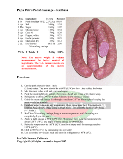

© Copyright 2026