
econstor
econstor
www.econstor.eu
Der Open-Access-Publikationsserver der ZBW – Leibniz-Informationszentrum Wirtschaft
The Open Access Publication Server of the ZBW – Leibniz Information Centre for Economics
Stimpfle, Alexander; Stadelmann, David
Conference Paper
The Impact of Fundamental Development Factors on
Different Income Groups: International Evidence
Beiträge zur Jahrestagung des Vereins für Socialpolitik 2015: Ökonomische Entwicklung Theorie und Politik - Session: Trade, finance and institutions, No. E08-V1
Provided in Cooperation with:
Verein für Socialpolitik / German Economic Association
Suggested Citation: Stimpfle, Alexander; Stadelmann, David (2015) : The Impact of
Fundamental Development Factors on Different Income Groups: International Evidence,
Beiträge zur Jahrestagung des Vereins für Socialpolitik 2015: Ökonomische Entwicklung Theorie und Politik - Session: Trade, finance and institutions, No. E08-V1
This Version is available at:
http://hdl.handle.net/10419/113128
Nutzungsbedingungen:
Die ZBW räumt Ihnen als Nutzerin/Nutzer das unentgeltliche,
räumlich unbeschränkte und zeitlich auf die Dauer des Schutzrechts
beschränkte einfache Recht ein, das ausgewählte Werk im Rahmen
der unter
→ http://www.econstor.eu/dspace/Nutzungsbedingungen
nachzulesenden vollständigen Nutzungsbedingungen zu
vervielfältigen, mit denen die Nutzerin/der Nutzer sich durch die
erste Nutzung einverstanden erklärt.
zbw
Leibniz-Informationszentrum Wirtschaft
Leibniz Information Centre for Economics
Terms of use:
The ZBW grants you, the user, the non-exclusive right to use
the selected work free of charge, territorially unrestricted and
within the time limit of the term of the property rights according
to the terms specified at
→ http://www.econstor.eu/dspace/Nutzungsbedingungen
By the first use of the selected work the user agrees and
declares to comply with these terms of use.
The Impact of Fundamental Development Factors on
Different Income Groups: International Evidence
February 2015
Abstract:
We jointly analyze the causal effects of geography, trade integration, and
institutional quality on different income groups for developing and developed
countries from 1983 to 2012. Favorable geographic conditions tend to
discriminate strongly between income groups as low incomes benefit whereas
high incomes decline. Controlling for institutional quality and geography, trade
integration has a negative effect which increases in absolute size and significance
for higher income groups. Institutional quality strongly and positively affects all
income groups, however, high income groups tend to profit relatively more than
low income groups. These findings are robust for different specification tests and
they are consistent over time.
Keywords: Economic growth, Inequality, Income Percentiles, Development
Economics.
JEL Classification: O11, O43, F43
I.
INTRODUCTION
Geographic conditions, trade integration and institutional quality are frequently
advanced as causal factors for economic development and growth (see, e.g., Diamond,
1997; Sachs, 2001; Frankel and Romer, 1999; Dollar and Kraay, 2004, Acemoglu et
al., 2001; Rodrik et al., 2004). As differences in average income levels between
developed and developing countries are enormous, the identification of fundamental
drivers for economic development has received central attention in economic debates.
At the same time, there are ongoing discussions on a widening of the income gap
between the rich and the poor in both developing and developed economies. After
Kuznets’ (1995) seminal work, a voluminous literature has emerged which analyzes
the link between income inequality and growth (see, e.g., Barro, 2000; Milanovic,
2005; Easterly, 2007). Looking at political debates, many fear that the rich may
benefit disproportionally from a nation’s overall economic advancement. While the
received literature has come up with different fundamental development factors and
intensely explored average growth and inequality, the effect of such fundamental
factors on different income groups has received relatively little attention. The paper
aims to fill this gap.
We analyze whether exogenous changes in geographic conditions, trade
integration and institutional quality favor or disfavor specific income groups relatively
more than others. Thereby, we advance the literature which analyzes fundamental
factors of economic development on average incomes. Instead of analyzing whether
we can attribute different average incomes across countries to differences in
geographic conditions, trade and institution, we analyze whether and how these
variables causally affect low and high income groups within countries.
To analyze this question we take a deliberately detailed perspective that
systematically looks at the effects of the fundamental factors established in the
literature on different income groups over 30 years. We construct a dataset of income
deciles for 138 countries which incorporates income distribution data from the latest
World Income Inequality Database. We then apply the established empirical crosscountry growth methodology on our dataset and we employ the development factors
which are analyzed in the recent literature for our econometric analysis. In particular,
2
we use the established instruments for trade integration and institutional quality to
ensure that our results can be causally interpreted.
The findings tend to confirm the related literature results for average income
levels. However, we find important differential effect of the variables on low versus
high income groups. Geographic conditions seem to discriminate between income
groups, which is evidenced in a consistent pattern of decreasing coefficients as we
move from low to high income groups. The influence of favorable geographic
conditions turns even negative once we passed the mean income group, indicating that
the poor are affected most by equator proximity. This pattern of results is broadly
consistent with views proposed by Sachs (2001). Trade integration has a negative but
often insignificant effect on all income groups which is similar to the negative
average impact shown be Rodrik et al. (2004). However, we tend to find that negative
effects as well as the significant levels increase for higher income groups. Hence,
trade has an equalizing effect across income groups. Institutional quality is associated
with systematic and large income gains for all groups at high statistical significance
levels. However, the effect of good institutional quality displays an increasing
coefficient so that high income groups seem to profit more than the poor from
institutional improvements. Overall, results are consistent over time, and we observe
that the model is relatively better in explaining lower incomes. We test the effect of
additional control variables, discuss methodological concerns, and perform a number
of validity tests. All robustness tests confirm the central results.
The remainder of this paper is structured as follows: Section 2 provides a
detailed literature review. We present the data and the estimation strategy in Section
3. Empirical estimation results for different income groups are presented in Section 4
and we perform robustness tests in Section 5. Section 6 offers concluding remarks.
II. LITERATURE REVIEW
A number of papers in a small but growing empirical cross-country literature
have looked at the effects of development factors on inequality (for a literature survey
in this field, see also Lopez, 2004). In particular, the influences of trade, sectorial
composition, and public policies on inequality have been thoroughly studied. In a
3
panel data set over 28 years, Spilimbergo, Londoño, and Székely (1999) find that
trade openness reduces inequality in capital-abundant countries, but increases
inequality in skill-abundant countries. Lundberg and Squire (2003), however, analyze
that a switch from zero to one in the dummy variable of the Sachs-Warner openness
indicator1 is associated with a 9.5 point increase in the Gini index, with significance
at the 10% level. Jaumotte, Lall and Papageorgiou (2013), using a newly compiled
panel of 51 countries over a 23-year period from 1981 to 2003, assign a greater impact
for inequality on technological progress than globalization i.e. openness to trade.
Globalization effects are offsetting one another because trade globalization is
associated with a reduction in inequality, but foreign direct investment leads to an
increase in inequality.
Lopez (2005) finds for his sample of 14 country case studies that inequality is
mainly driven by the people employed in the non-agricultural sector. Hence, when this
sector does well, inequality tends to increase. When this sector underperforms (as it
did during the 1980s when non-agricultural growth was below agricultural growth)
inequality would tend to decline with growth. Ravallion and Datt (2002) observe a
similar pattern for India, where non-farm growth is a strong factor for reducing
poverty. However, the actual effects are highly region-dependent, and success
depends on initial rural and human resource development as well as egalitarian land
distribution. Easterly (2007) confirms that agricultural endowments predict inequality.
For a regional study on Africa, Odedokun and Round (2004) concluded that regional
dummies, overall size of the government, and lack of skilled manpower as significant
inequalizing variables. However, their results when testing effects of international
openness to trade on inequality turn out to be non-significant.
In the realm of public policy, Milanovic (2000) finds evidence that inequality is
actively steered by social choice variables (social transfers and state sector
employment), which decrease inequality on average by some 13 Gini points. He
1
The Sachs-Warner dummy is a variable that classifies an economy as closed if it is closed according to
any one of the following five criteria: (a) average tariff rate exceeded 40%, (b) non-tariff barriers covered
more than 40% of imports, (c) a socialist economic system (d) a state monopoly of major exports, or (e)
black-market premium exceeded 20% during either the decade of the 1970s or the decade of the 1980s.
4
argues that the preference for social equality is income-elastic so that social choice
variables play a more prominent role as the nation gets wealthier. Results by Checchi
et. al. (2008) indicate that stronger labor market institutions are correlated with lower
inequality, with the notable exception of the tax wedge that exhibits a positive
correlation with the Gini coefficient. There is also empirical evidence that more
democratic countries, better enforcement of the law, and financial development are
associated with higher income equality, while a more segmented labor market and
lower union density are correlated with greater inequality (Barro, 2000; Bourguignon
and Morrisson, 1998; Li, Squire and Zou; 1998; Alderson and Nielsen, 2002).
While important contributions, most of this literature is relatively mute on factors
driving incomes of specific income groups in a country, so that changes in overall
inequality cannot be traced down further. In contrast, astonishingly few papers
analyze the effect of fundamental factors for economic growth on different income
percentiles within a country2. Usually such research focuses on the bottom income
groups. White and Anderson (2000) report that growth associated with progressive
distributional changes will have a greater impact in raising poor incomes than 'general'
growth which leaves distribution unchanged. Redistributional strategies matter in
particular since for around every fourth case they examine, distribution has been
equally important as growth for explaining income growth of the poor.
Another important stream of literature takes the stand that most of the variation
in changes of bottom incomes can be attributed to the growth rate of average incomes.
Dollar and Kraay (2002) focus on the effects for the bottom 20 percent of the income
distribution, applying the regressors openness to international trade, macroeconomic
stability, moderate size of government, financial development, and strong property
rights and rule of law. They do not find a systematic relationship between any of these
variables and the poorest quintile and conclude that the poor benefit equiproportionately from growth determinants like everyone else in society. Dollar et al.
(2013) expand this work in a dataset spanning 118 countries and four decades. They
2
Grossmann and Stadelmann (2013), for instance, examine the wage effects for specific income groups
(80th and 90th percentile) migrating from developing countries to advanced economies. This paper,
however, has a within-country focus and disregards effects from international mobility.
5
re-confirm the essential outcome that incomes of the bottom 20 percent and bottom 40
percent of the income distribution generally keep in step with a rise in average
incomes.
Work by Kray (2006) and Dollar et al. (2014) echoes these findings. The latter
find, through a Bayesian Model Averaging, that there is little empirical evidence that
any of their 13 growth variables3 are robustly correlated with the income share of the
bottom 40 percent. In conclusion, they underscore the pivotal role of rapid growth in
average incomes because thereby the poor benefit most as well.
However, Balakrishnan, Steinberg, and Syed (2013) report deviating findings
when applying the same methodology to Asian and Latin American countries, but
instrumenting the dependent income variable4. In a rare research specification which
aims to analyze both poor and rich income groups, they find that the bottom quintile
participated less than proportional in average income growth while the top quintile
participated over-proportionally. The authors also emphasize significant result
differences across regions. Overall, education, industry employment, and financial
inclusion reforms appear as pro-poor and inclusive growth variables. On the other
hand, financial openness seems to be negative for the bottom income brackets.
Roine, Vlachos, and Waldenström (2009) study economic determinants which
are particularly pro-rich. They find that periods of high economic growth, and
financial development, measured as the relative share of the banking and stock market
sectors, benefit the top income bracket disproportionally. In contrast, government
spending and openness to trade have no clear effects on the rich, with the latter even
tilting towards a negative effect.
3
4
These are measure of financial development (M2 as percentage of GDP), the Sachs-Warner indicator of
trade openness, the Chinn-Ito Index of financial openness, the inflation rate, the general government
budget balance, life expectancy, population growth, the Freedom House measure of civil liberties and
political rights, the frequency of revolutions, and a dummy variable indicating whether the country was
party to a civil or international war in a given year, primary school enrollment rates, a measure of
educational inequality, and the share of agriculture in GDP.
Specifically, they use lags of real per capita income as measured in the Penn World Tables (PWT) to
instrument the household-survey-based average income variable. The authors argue that “the lagged
variables help correct for endogeneity bias by identifying the component of income that is
predetermined, and the PWT measure of income help corrects for measurement error by identifying the
component of income as measured by the household survey that is also consistent with this secondary
measure of income” (ibid., p.9).
6
The analysis of growth variables for different income groups to find out if effects
differ for poor or rich uses a different angle for examining the growth inequality
nexus. While there has been valuable work already in this field, the literature review
identified a set of open research gaps. There has not been so far a detailed global
effort to systematically analyze the effect of fundamental growth factors on both the
rich and the poor. Most of the empirical work presents itself as rather scattered, with
key growth regressors and/or income groups missing, and with explanatory variables
employed that make it hard to identify a common systematic pattern. Also, there is
very limited knowledge whether the role of development factors changes for specific
income groups over time. Effects have been mostly estimated for only one point in
time, and hence, results are susceptible to time-variant effects.
In this paper, we provide a detailed perspective on all key income percentiles to
determine how growth variables affect different parts of society, from the very poor to
the very rich. Estimates are also repeated for several time periods to address potential
outliers. This design is targeted to recognize the need to go beyond a narrow view
definition of development, measured through average incomes only. It thereby
incorporates the aspect that certain development factors may be considered preferable
if they favor the poor, or at least lead to higher incomes throughout all parts of society.
III. DATA AND IDENTIFICATION
STRATEGY
Data
We newly construct income deciles for 1385 countries by combining information
on average national income per capita reported by the Penn World Tables 8.0
(Feenstra, Inklaar, and Timmer, 2013) with the most recent data on income dispersion
from the UNU-WIDER database (2014a). The literature on cross-country growth
regressions warns us of the pitfalls in “just merging” data from different sources
(Atkinson and Piketty, 2007). We follow the argumentation of Dollar and Kraay
(2002) who point at the pragmatic advantages of incorporating per capita GDP data
5
As many of these 138 countries have only selected data entries over the timespan under investigation, no
time period sample has all 138 countries included simultaneously. The maximum sample size is 117.
7
for income distribution data, namely better data availability and enhanced
comparability with existing literature. Therefore, for the average income level
measurement, we apply the real GDP per capita data at current PPPs from the Penn
World Tables. Sala-i-Martin (2006), too, advocates our approach of merging national
account (Penn World Tables) and survey (UNU-Wider) inequality data. Roine et al.
(2009) base their income measurement on personal income tax returns (for a similar
methodology see also Piketty and Saez, 2003; Atkinson, Piketty and Saez, 2011).
Ideally individual income tax data would be used also in this paper to construct
income deciles. However, even such data may suffer from tax avoidance and evasion
(Atkinson and Piketty, 2007; Davies et al., 2007; Leigh, 2007) and, more importantly,
reliable data is not available for a sufficiently large number of countries, in particular
less-developed countries.
The UNU-WIDER database on income dispersion by the United Nations
University builds on previous work by Deininger and Squire (1996). The revision
WIID3b used here contains data for developed, developing, and transition countries.
Released only in summer 2014, it represents an enhanced level of data availability
with the latest observations now reaching the year 2012 (UNU-WIDER 2014b). It also
responds to earlier criticism regarding quality and consistency (Atkinson and
Brandolini, 2001, 2009), for example by closely following the recommendations of
the Canberra Group (2001) for developing international standards for income data.
The break-down of the UNU-WIDER income distribution data is generally limited to
the decile level. As the heterogeneity of the top decile has frequently been pointed out
(Atkinson et al., 2011; Piketty, 2014; Roine et al., 2009), data on the top one percent
or top five percent would have potentially provided additional valuable insight.
However, as the focus here is to examine the macro-effect of development factors
across various income groups from poor to rich in lieu of an exclusive top income
study, we regard the given dataset as sufficient. Furthermore, the heterogeneous
character of the very rich would make an econometric modeling of their incomes
nearly impossible, since people mostly attained such high incomes by individual
factors beyond the fundamental growth factors.
8
A set of five-year timespans will be the subject of analysis. If there is at least one
data point available per timespan for the income bracket under scrutiny, the respective
country is included in the data set. No data points are constructed if they are not
available. In case of several data points per period, we apply a simple average of the
years with available data. A detailed overview of the countries which form the
respective sample per time period can be found in the appendix. If there were several
sources for the same single year and country available in the UNU-Wider database,
we used the one with the most data points across all percentiles to enter the average
calculation of the given time period. Then, for calculating the dependent variable
Income Di (income of a population decile for country i), we multiply the average
national income per capita yavgi with the given decile share Di divided by respective
decile d:
(1)
Income Di = (Di/d) • yavgi
At the country level we explain income levels by a set of three variables. GEOi,
TRADEi, and INSTi are respectively country measures for geography, trade
integration, and institutions. This core regression specification is closely aligned with
the choice of variables by Rodrik et al. (2004) who employ these three fundamental
development factors, which they refer to as the “three strands of thought [that] stand
out” (p. 132) for determining whether societies develop or not6. The three explanatory
variables hence represent development factors which are widely regarded as most
fundamental for development (see for example Barro, 1991; Diamond, 1997; Gallup
et al., 1998; Sachs, 2001; Sachs and Warner, 1995; Frankel and Romer, 1999; Hall
and Jones, 1999; Acemoglu et al., 2001, 2002, Sala-i-Martin et al., 2004).
The concrete choice of variables to represent the respective fundamental factor is
then based on their acceptance in the literature as well as their level of data
availability for our specific set of countries. Institutional quality is measured by World
Bank data on “Rule of Law” which reflects perceptions of confidence in rules of the
society, including quality of contract enforcement and property rights. This measure
can take values from -2.5 (weakest institutions) to +2.5 (strongest institutions)
6
Rodrik et al. (2004) call them "deeper determinants" as opposed to the term "fundamental development
factors" used in this paper, but the underlying idea is basically the same.
9
(Kaufmann et al., 2002). We instrument this endogenous variable by Hall and Jones’
(1999) fraction of the population speaking English and other European languages.
These language data were originally used by the authors to construct an aggregate
social infrastructure index.
Rodrik et al. (2004) proceed with a very similar
methodology by using the Hall and Jones language data as instrument for institutions
in order to expand their sample.
Trade integration is measured by the share of exports and imports combined of
national GDP, using World Bank data7. The variable is instrumented by Frankel and
Romer’s (1999) constructed trade shares, a method that has passed the 'American
Economic Review (AER)-test'. The authors compute predicted values of bilateral
trade based on geographical features, and allocate these bilateral trade flow
coefficients also for country pairs which are not included in their original sample. This
has caused criticism as to the weakness of their instrument and a call for more explicit
geography controls (Noguer and Siscart, 2005). Thus, we account for the variable
geography in the regression equation separately. The remaining explanatory variables
geography is expressed through "distance from equator". In robustness tests we will
also include alternative geography variables.
Table 1 provides descriptive statistics for the key variables and the respective
periods of analysis. Improvements in data availability are reflected in the increase of
the sample size over time from 56 countries in the 1985 set (measured as average of
1983-1987) to 117 countries in the 2005 set (measured as 2003-2007). The average
real GDP per capita income in our sample has risen by 64 percent (from $5,454 to
$8,968) between 1985 and 2010, which corresponds to a compound annual growth
rate of 2.0 percent.
This falls short of the actual reported global per capita income
growth of 2.9 percent p.a. during that period (World Bank, 2014).
7
Here we also closely follow Frankel and Romer (1999) who use the current price local currency tradeGDP ratio reported in the Penn World Table, although there are other methods proposed. Alcalá and
Ciccone (2004), for example, provide a careful theoretical justification for PPP-adjusted trade ratio as a
measure of trade openness.
10
Table 1: Descriptives
Sample size
Log Income First Quintile
Log Income Median
Log Income Average Population
Log Income Top Quintile
Log Income Top Decile
Geography (GEO_disteq)
Log Trade Openness (LN_Trade_WB)
Institutions (Inst_Rule_of_Law)
1985
56
7.27
(1.32)
8.29
(1.22)
8.60
(1.08)
9.45
(0.98)
9.72
(0.94)
0.34
(0.19)
3.93
(0.60)
0.39
(0.98)
1990
71
7.16
(1.56)
8.17
(1.36)
8.52
(1.21)
9.38
(1.10)
9.67
(1.06)
0.31
(0.19)
3.99
(0.51)
0.19
(1.01)
1995
107
7.08
(1.52)
8.10
(1.35)
8.47
(1.21)
9.35
(1.12)
9.65
(1.08)
0.33
(0.19)
4.15
(0.53)
0.03
(0.95)
2000
97
7.27
(1.52)
8.26
(1.37)
8.58
(1.27)
9.43
(1.20)
9.72
(1.18)
0.33
(0.20)
4.23
(0.51)
0.05
(0.98)
2005
117
7.43
(1.5)
8.34
(1.43)
8.64
(1.35)
9.47
(1.28)
9.74
(1.27)
0.31
(0.20)
4.36
(0.52)
0.04
(1.00)
2010
91
7.93
(1.42)
8.84
(1.34)
9.10
(1.25)
9.90
(1.18)
10.17
(1.15)
0.35
(0.20)
4.38
(0.55)
0.22
(1.04)
This is due to the limited data availability in early periods which biases our first
samples towards higher income countries. Indeed, the 56 countries’ average income
level is about twice the average global income for 1985. This higher jump-off point
leads to a smaller subsequent growth rate until 2010, where the annual per capita
income of our gradually increased sample and the actual global income levels
converge at around $9,000.
A granular view of the sample data at hand reveals that, over the 25 years, the
bottom 20 percent of the income distribution have actually grown disproportionally by
2.7 percent per annum, while the wealthiest 10 percent saw their incomes increase by
only an annual 1.8 percent. Mere income level trends hence suggest a converging
trend of incomes, albeit at a slow pace. In absolute figures, in 2010 the average global
top 10 percent income of $26,140 was still over nine times the $2,788 reported for the
bottom 20 percent; in 1985, this top-to-bottom ratio had even been close to 12. For the
input variables, we can observe a reduction of institutional quality over the timeframe
by 16 percent, whereas the sample’s average geographic dispersion remained constant.
Trade volumes see a sizeable hike over the years, growing at almost 2 percent p.a. for
our dataset.
11
Identification and estimation strategy
Given the data structure, the first step of the estimation procedure is to analyze a
series of regressions in which the log of income deciles are related to fundamental
development factors. . Hereby, we are interested in the respective variable coefficients
and their variation depending on the percentile income per capita examined. The basic
econometric model is as follows:
(2)
ln [ 𝐼𝑛𝑐𝑜𝑚𝑒𝐷𝑖 ] = µ + αGEOi+ β TRADEi + γ INSTi + εi
I address the challenges in measuring the variables institutions and trade as truly
exogenous factors for income through a two-stage least squares estimation (2SLS)
procedure. We resort to well-established and commonly used existing instrumental
variables (amongst others see Rodrik et al., 2004; Alcala and Ciccone 2004; Dollar
and Kraay 2003).8
In the first-stage regressions of the 2SLS equation, institutions INSTi and trade
integration TRADEi are regressed on all exogenous variables which yields:
(3)
INSTi = θ + σLANGi + πCONSTRAi + ωGEOi + εINSTi,
(4)
TRADEi = λ+ ϕ LANGi + ξCONSTRAi + νGEOi + εTRADEi,
where LANGi refers to language data of Hall and Jones (1999), and CONSTRAi
to constructed trade shares by Frankel and Romer (1999). The exclusion restrictions
require that LANGi and CONSTRAi do not appear in equation (2).
With the described variables at hand, the estimated slope coefficients capture the
partial correlations between the set of regressors and the different income groups.
Specifically, we analyze the average GDP per capita, the bottom 20 percent (20th
percentile), the median (50th percentile), the top 20 percent (80th percentile, and the
top ten percent (90th percentile) of the income distribution. For example, let us assume
that the variable trade integration had a positive coefficient for the bottom 20 percent,
but a negative coefficient for the top ten percent. If we then take a specific case, say
Nigeria, the coefficient sign of the average GDP per capita would help us understand
the overall direction and effect of the trade variable for this country.
8
There is a literature which discusses shortcomings of these standard instruments (see Eberhardt and Teal,
2011; Deaton, 2010; Bazzi and Clemens, 2013; amongst others). We will deal with major issues when
analyzing the robustness of our results.
12
We run the regression on a set of different 5-year timespan averages to identify
robust patterns and to spot potential historical outliers in order to put the findings on a
broader basis. The resulting analysis represents a step beyond the usual single cross
section analysis conducted so far. There are only selected cases for using panel data in
this field of research (see for example Irwin and Terviö, 2002 or Dollar, Kleineberg
and Kraay, 2014). We start with the 5-year average around 1985 (1983-1987) as this
represents the earliest sensible data set available. This is then repeated analogously
from 1988-1992, 1993-1997, 1998-2002, 2003-2007, and finally 2008-2012.
The regressor GEOi as well as the instrumental variables LANGi and
CONSTRAi remain constant over the various periods. While trade shares on the basis
of Frankel and Romer’s methodology could be constructed also for other time periods
than their base year 1985, there are a number of reasons to refrain from doing so.
First, the constructed trade shares are calculated using geographical variables which
remain generally constant, in particular over our limited timeframe of 30 years.
Hence, there will be very little data variation even with an elaborate re-creation of
trade shares for other years. Second, this conceptual consideration is underpinned by
empirical work from Feyrer (2009). He introduces a dynamic instrument for trade on
the basis of Frankel and Romer, which results in a close confirmation of their findings.
Frankel and Romer’s instrument is quite robust over time. Third, Rodrik et al. (2004)
also decide to keep trade shares as a constant instrumental variable with the original
1985 values, even when using them to estimate 1995 GDP per capita values. Hence,
theory, empirics, and recognized literature point us towards using fixed values for
CONSTRAi. For most time periods of our data set, the 1985 values are consequently
lags which may be even considered preferable from an exogeneity perspective. INSTi
and TRADEi, in contrast, will be dynamically adjusted to the respective period.
To increase the validity of our regressions, we examine samples with the
respectively largest number of country data available per time period, which will
result in larger sample sizes as we move towards the present. Unfortunately, a number
of countries from the former Eastern bloc are not included. This is due to missing
income distribution data as well as territorial re-organizations which affect
13
comparability over time. Nonetheless, most of the larger countries such as Russia,
Poland or Romania could be included in the analysis.
IV. EMPIRICAL RESULTS
Baseline OLS results
We start with simple correlations to investigate in how far generally our input
variables and the different income levels move together. Figure 1 contains a scatter
plot for 2005. The first look at the data reveals that geography (distance from equator)
shows a correlation coefficient of around 0.7 with income, and clearly higher
correlation displayed for the poor deciles vis-à-vis the rich deciles. As reflected in the
scatter plot, trade on the other hand show a rather weak correlation, which only
somewhat increases over the years from roughly 0.2 to 0.3. We cannot observe an
income-related pattern. Finally, institutional quality is highly correlated to incomes,
roughly at 0.8. We also observe a slight but persistent correlation pattern across
income levels, with higher coefficients for the poor than for the rich. In summary,
income of the poor correlates more strongly with geography and institutions than
income of the rich. Trade plays a secondary role in this context, and has no distinct
correlation dynamics depending on the income groups.
Next, we look at the way the described bivariate relationships between variables
are mirrored in a simple OLS regression of equation (2). Results are summarized in
table 2 across income levels, exemplified again for 2005. First evidence (without
taking account of causality issues) generally confirms the literature’s findings (in
particular Rodrik et al., 2004) with regard to the sign and significance levels of
variables. These hold also true for most of the income distribution examined, with
exceptions identified at the top end. Therein, geography tends to lose its significance
and the coefficient is on average only one third of its value for the bottom quintile. We
also observe a modest decline of the coefficient size for institutions as we go from
poor to rich. In general, the coefficient pattern follows a linear trend so that inspection
of top and bottom income groups allows to also draw conclusions about median and
14
average. There are no peculiarities around the middle income groups that require
additional interpretation.
The R-square decreases as we move from poor to rich income segments. Hence,
incomes of the poor can be more precisely estimated with the variables at hand than
income of the rich. Results are qualitatively similar also for the other time periods,
with the caveat that trade point estimates are never very precise.9. Altogether,
countries more distant from the equator and stronger institutions are likely to have
higher incomes. Geography generally displays high significance, except for selected
time periods when both looking at top income groups and simultaneously controlling
for institutions. Institutions in return are always significant at the one percent level and
give a boost to the overall level of regression fit.
9
Trade displays relatively large standard errors which lead to non-significant coefficients. The coefficient
sign is consistently positive only from the year 2000 onwards. An overview of OLS results across time
periods is given in the appendix.
15
COD
0.00
(
0.20
COD
4.00
0.40
GEO_disteq
LN_Trade_WB
LSO
LUX
5.00
0.60
LUX
LUX
0.740
0.80
6.00
r= 0.279
HKG
SGP
NOR
ISL
AUT NLD
CHE
IRLDNK SWE
FRA BEL
DEUGBR CAN FIN
AUS
SGP
JPN
TAI
CYPUSA
ESPITA SVNCZE
GRC
SVK
HUN
PRT
ISR
EST
HKG
MUS
POL LTU
KAZ BLR LVA
RUS
GAB
IRN
BGR
UKR
MYS
TUR
MEX
ROU
CHL
THA
URY
ARG
VEN
CRI
EGY
TUN
UZB
DOM
JOR CHN ARM
MKD
PAN
JAM
BWA
BRA
LKAPER
IRQ
GEO
ECU
COL
PAKSYR
FJI
BTN
ZAF
KGZ MDA
VNM
PHL YEM
NAM
PRY
COG GHA KHM
GTM MRT
SENBOLIND
BEN
ZMB
BGD
HND
TZA NGA
NPL
KEN TGO
GIN
UGA
GMB MLI
RWA ETH BFA
SLV MDG
MWI
LSO
NER
CAF
r=
LBR COM MOZ
Quintile 1
b)
(
NOR
ISLSWE
AUT NLD BEL
DNK
IRL
FINCHE
FRA CANDEU
AUS
JPN
GBR
SVN
USA
CYP TAI
CZE
ITAESP
GRC
SVK
HUN
PRT
ISR
EST
LTU
MUS
POL
KAZLVA BLR
RUS
IRN
GAB BGR
UKR
TURMEX CHL
MYS
ROU
THA
URY
ARG
VEN
EGY
TUNCRI
UZB
DOM BWA
CHN
PAN
JAMMKD JOR
BRA
LKAGEO
IRQ
PER ECU ARM
PAK
COL
SYR
FJI
ZAF BTN
KGZ MDA
VNM
PHL
YEMNAM
GHA PRY
COG
MRT
GTM
KHM
SEN
BEN BOL
IND
ZMB
BGD
NGA
HND
TZA TGO
KEN
GIN
UGANPL
MLI GMB
BFA
MDG
RWA ETH
SLV
MWI
LSO
CAF NER
MOZ
LBR
COM
3.00
c)
IRQ
LBR
COM
-1.00
NER
MOZ
0.00
Inst_rule_of_law
1.00
2.00
r= 0.802
NOR
ISL
SWE
AUT
CHE
DNK
NLD
FIN
BEL IRL
DEU
AUS
CAN
SGP
JPNFRA
GBR
SVNTAIESP
USA
ITA CZECYP
SVK GRC
HUN PRT
ISR
EST
HKG
POLLTU MUS
BLR KAZ
LVA
RUS
IRN GAB BGR
UKR
MYS
TUR
ROU
MEX
CHL
THA
URY
ARG
VEN
CRI
EGY
TUN
UZB
DOMMKD
JOR BWA
PAN
CHN
JAM
ARM
LKA
PER BRA
ECU
SYR
COL
PAKGEO
FJIBTN
MDA
ZAF
KGZ
VNM
PHL
YEM
NAM
PRY
GHA
COG KHM
MRT
GTM
BOL BEN
SEN IND
ZMB
NGA BGD
HND
TGO
NPL UGATZA
KEN
GIN
GMB
MLI
BFAMDG
ETH
SLV
RWA
MWI
CAF
COD
COD
0.00
(
(
0.20
COD
4.00
0.40
GEO_disteq
LN_Trade_WB
LUX
5.00
0.60
NOR
USA
IRL
CHE
ISL
DNK
AUT NLD BEL
AUS
CANDEU
FINSWE
GBR
FRA
JPN
ITA
ESP
CYP TAI
SVN
GRC
CZE
PRT ISR
HUNSVK
LTU EST
POL
LVA
RUS
BLR
TURMEX
IRN CHL
KAZ BGR
MUS
ROU GAB
MYS
ARG
MKD
VEN
URY
BWACRI
UKR PAN
THA
BRA
DOM TUN
CHN
COL PER ECU
JAM
EGY ARM
UZB GEO
FJI
JOR
IRQ
ZAF LKA
GTM
BTN
PRY
PHL
MDA
BOL SYR
VNM
PAK
YEMNAM KGZ HND
COG
IND
GHAMRT
NGASEN
KHM
ZMB
BGD BEN KEN SLV
GMB
TZA
LSO
GIN
UGANPL
MLIMDG TGO
BFA
RWA
MWI
COM
CAF NER
ETH
MOZ
LBR
3.00
COD
-1.00
0.00
Inst_rule_of_law
1.00
LUX
r= 0.711
0.80
SGP
HKG
r= 0.281
6.00
2.00
r= 0.792
NOR
USA
IRLCAN
CHE
ISL
DNK
AUT
NLD
SWE
SGP
AUS
BELFRA
DEU
FIN
GBR
JPN
ITA
HKG
TAIESP
CYP
SVN
GRC
ISR
CZE
PRT
HUN
SVK
EST
POLLTU
LVA
RUS
BLR KAZ
BGR TUR
IRN GAB
MEX ROU
MYS MUS CHL
ARG
MKD PAN
VEN
URY
CRIBWA
UKR
THA
TUN
BRA
DOM
CHN
COL
ECU PER
ARM EGYFJI JOR
UZB
GEOJAM
LKA
ZAF
GTM
BTN
PRY
PHL
MDA
SYR
BOL
NAM
VNM
PAK
KGZHND
COG YEM
GHAIND
MRT
SEN
KHM
NGA
BEN GMB
KEN ZMB
BGD
GIN
TGO
UGATZALSO
NPLSLV
RWABFAMDGMLI
MWI
COM ETH
MOZ
LBR NER
CAF
LUX
NOR
USA
IRLDNK CAN
CHE
ISL
AUT DEU
NLD
SGP
SWE
AUS
FIN
GBR
JPNESPITA FRA BEL
HKGTAI
SVN
ISR CYP GRC
CZE
PRT
HUN
SVK
EST
POL LTU
LVA
RUS
BLR
IRN
MEX
GAB
MUS
MYS
ROU CHL
ARG TUR BGR KAZ
MKD
VEN
URY
CRI THA
PAN
BWA
UKR
TUN
BRA
DOM
CHN
COL PER
ECU
JAM
EGY JOR
ARM
UZB
FJI
GEO
LKA
ZAF IRQ
GTM
BTN
PHL VNM
MDA
BOL PRY
PAKSYR
YEM NAM
KGZ
HND
COG
IND
GHA SEN MRT
BENNGAKHM
ZMB
KEN TZA
BGD
GMB
SLV
LSO
GIN
UGA TGO
NPL
BFA MLIMDG
RWA
MWI
CAF ETHCOM
NER
MOZ
LBR
Median
e)
f)
IRQ
-2.00
COD
0.00
(
(
0.20
COD
4.00
0.40
GEO_disteq
LN_Trade_WB
5.00
0.60
NOR
USA
CHE
IRL
AUS
ISLSWE
AUT NLD BEL
GBR CANDEU
JPN
FIN DNK
FRA
ITAESP
ISR CYP TAI
GRC
SVN
CZE
PRT
HUN
EST
SVK
LTU
POL
RUS CHL
LVA
MYS
TURMEX
GAB
ARG
IRN
BWA
MUS
BLR
PAN
URY ROU KAZ
CRI BGR
VEN
BRA
ZAF DOM
MKD THA
COL
TUNUKR
PER ECU CHN
JAM
FJI
NAM
ARM
UZB GEO
EGYGTM
JOR
PRY
BTN
LKA
BOL
PHL IRQ
HND
SYR
MDA
COG
VNM
PAK IND
YEM
KGZ
GHAMRT
KHM
NGASEN
ZMB
BGD BEN
GMB
KEN
LSO
UGANPL
COM GINSLV
RWA
TZA TGO
BFA
MLIMDG
CAF NER
MWI
MOZ
ETH
LBR
3.00
COD
-1.00
0.00
Inst_rule_of_law
1.00
0.683
0.80
SGP
HKG
r= 0.270
6.00
LUX
2.00
NOR
USA
CHE
IRLCAN
ISL
AUS
SGP
NLD
AUT
DNK
GBR
SWE
BEL HKG
DEU
JPN
FIN
ITA
TAIESP FRA
ISR
CYP
GRC
SVN
CZE
PRT
HUN
EST
SVK
POLLTU
RUS
LVA
MEX
CHL
MYS
TUR
ARG GAB BGR
BWA MUS
PAN
BLR KAZIRN
ROU
CRI
URY
VEN
BRA
THA
ZAF
DOM
COLMKD
TUN
UKR
PER
ECU
CHN
JAM
FJI
NAM
UZB GTM
GEOARM EGY
JOR
PRY BOL
BTN
LKA
PHL
HND
SYR
IND
COG YEM PAK MDA
VNM
KGZ
GHA
MRT
KHM
SEN
NGA
BEN GMB
BGD
KEN ZMB
LSO
SLV
NPL
UGATZA
RWA
GIN COM TGO
BFAMDGMLI
r= 0.786
MWI
NER
MOZ
ETH
CAF
LBR
LUX
NOR
USA
CHE NLD
IRL
ISL
SGP
HKG AUS
AUTBEL
DNK CAN
SWE
JPNESPITA FRA
DEUGBR
FIN
TAI
ISR CYP GRC
PRT SVNCZE
HUN
SVK
EST
LTU
RUS POL LVA
MEX
CHL
MYS
GAB
IRN
ARG TUR BGR KAZ BLR
BWAROU
PAN
MUS
CRI
URY
VEN
BRA
THA
ZAF
DOM
MKD
COL
TUN
UKR
PER
ECU
CHN
JAM
FJI NAM
ARM
UZB
GEO
EGY JOR
LKA PHL GTM
BOL PRY BTN IRQ
HND
SYR
MDA
COG
VNM IND
PAK
YEM
KGZ
GHA
MRT
SEN
NGAKHM
ZMB
BGD LSO
GMB
KEN BEN
SLV
NPL
UGA
COM
RWA TGO
TZA GIN
BFA MLIMDG
r=
CAF
MWINER
MOZ
ETH
LBR
LUX
Average Population
h)
i)
IRQ
-2.00
Quintile 5
COD
0.00
(
0.20
COD
4.00
CAF NER
ETH
(
GIN
0.40
GEO_disteq
MOZ
MWI
LN_Trade_WB
0.60
0.638
0.80
HKG
SGP
5.00
LBR
6.00
r= 0.253
USA
NOR
AUS
GBR CANISL CHEAUT NLD IRL
JPN
BEL
ITA
ISR
DNK
SWE
TAI
FIN
FRA
ESP PRTDEU
GRC
CYP
SVN
CZE EST
MEX CHL
LTU HUNSVK MYS
POLBWA
TURRUS
ARG
GABLVA PAN
ZAF
IRN
BRA
URY ROU CRI
COL
VEN DOM
KAZ BGR
THA
MUS
BLR
PER ECU
NAM
TUN
CHN
JAMMKD FJI
UKR
GTM
ARM
BOL
BTN GEO PRY
JOR
EGY UZB
HND
LKA
PHL IRQ
IND
COG
SYR
MDA
VNM
YEM
PAK
KGZ
GHAMRT
KHM
NGASEN
LSO
GMB
BGD COM
ZMB
RWA
BEN KEN SLV
UGANPL
GIN TZA
BFA
MLIMDG TGO
3.00
COD
-1.00
0.00
Inst_rule_of_law
1.00
2.00
LUX
USA
HKG
NOR
IRL
CHE
AUS
CAN
GBR
ISL
NLDAUT
JPN SGP
BEL
ISRTAIESP
ITA
DNK
FIN
FRA DEUSWE
GRC
CYPPRT
SVN
CZE
EST CHL
MEX
BWA
RUS
LTU
SVK
MYS
POL
LVA HUN
PAN TUR
ARG
ZAF
IRN GAB
CRI
BRA
URY
ROU
COL
VEN
BGRTHA
DOM
MUS
BLR KAZ
ECU PER
NAM
TUN
JAM
CHN
MKD
FJI
GTM UKR
GEOARM
BTNJOR
UZB PRY BOL
EGY LKA
HND
PHL
IND
COG
SYR
MDA
VNM
YEM
KGZ PAKMRT
GHA
KHM
NGA COM
SEN
LSO
ZMB
BGD
KEN RWA
BEN GMB
SLV
NPL
UGA
BFATZA MLI
TGO
MDG
MOZ
MWI
NER
r= 0.764
LBR ETH
CAF
LUX
LUX
USA
HKG
NOR
CHE IRL
AUS
CAN ISL
SGP
GBR
NLD
AUTBEL
ISR JPNESPITA FRA
DEU
DNK SWE
TAI
FIN
PRT
CYP GRC
SVNCZE
EST
CHL
MEX
HUN
BWA
RUS
SVK POL LTU
MYS
LVA
PAN
ARG TUR
GAB
ZAFIRN
CRI
BRA
URY
ROU
COL VEN
BGR KAZ BLR
THA DOM
MUS
PER
ECU
NAM
TUN
JAM
CHN MKD
FJI
UKR
GTM
ARM
BOL PRY BTNJOR
GEO
UZB
EGY IRQ
LKA PHL HND
IND
COG
SYR
MDA
VNM
YEM
PAK
KGZ
GHA KHM MRT
NGA
SEN
COM
GMB
ZMB
BGD LSO
KEN
RWA BEN
SLV
NPL
UGA
BFA MLI
TZA GIN
TGO
MDG
CAF
MOZ
MWINER
r=
ETH
LBR
Top Quintile
k)
l)
IRQ
-2.00
Decile 10
COD
0.00
LBR
ETH
(
(
0.20
4.00
ETH
COD
0.40
GEO_disteq
LN_Trade_WB
LBR
5.00
0.60
LUX
0.612
0.80
6.00
r= 0.251
SGP
HKG
LUX
HKG
USA
NOR
CHE IRL
SGP
AUS
GBR CAN ISL
NLD
ISR JPN ITA AUTBEL
TAI
FIN
ESP FRA DEU DNK SWE
PRT
CYP GRC
CHL
MEX
SVN
CZE
EST
BWA
MYS
HUN
PAN
ZAF
TUR
RUS
SVK POL LTU
LVA
GAB
ARG
BRA
URY
IRN
COL CRI
DOM ROU
VEN
BGR KAZ
ECU
NAM
PER THA MUS
TUN
BLR
CHN
JAM
FJI
GTM
MKD
ARM
BOL PRY BTN
UKR
JOR
GEO
UZB
LKA PHL HND
EGY
IND
IRQ
COG
SYR
MDA
YEM
PAK
GHACOM
KHM MRT
NGA ZMB
LSO
GMB
SEN
BGD NPL
RWA
SLV
UGA
KEN BEN
BFAVNM
GIN
KGZ
MLIMDG
TGO
TZA
CAF
r=
MOZ
MWINER
Top Decile
n)
COD
-1.00
LBR ETH
0.00
Inst_rule_of_law
1.00
2.00
LUX
HKG
USA
NOR
IRL
CHE
CAN
AUS
SGP
GBR
ISL
NLDAUT
ISRTAI JPN
ITA
BELFRA DEUSWE
FIN
DNK
ESP
GRC
CYPPRT
CHL
SVN
MEX
EST
BWACZE
MYS
ZAF POL
RUS ARG GAB PAN TUR
SVKLTU
LVA HUN
BRA
CRI
URY
IRNCOL
DOM
VEN
ROU
BGRTHA
NAM
ECU PER
KAZ
MUS
TUN
BLR
CHN
JAM
FJI
PRY UKR
GTM
ARM
BOL MKD
BTNJOR
HND GEOPHL
UZB
EGY LKA
IND
COG
SYR
YEM PAK MDA
MRT
GHA
KHM
ZMB
NGA COM
LSO
GMB
SEN
BGD NPL
RWA
SLV
BEN
UGA
KEN
VNM
BFA
GIN KGZ
TGO
MDGMLI
TZA
r= 0.757
MOZ
MWI
NER
CAF
USA
NOR
IRL
AUS
GBR CAN CHE
ISL
JPN
ISR AUTTAINLD BEL
ITA
FIN
FRA
DNK
ESP PRTDEU
SWE
GRC
CYP
MEX CHL
SVN
CZE EST
BWA
HUNSVK MYS
TURRUS
ZAF
POL GABLVALTU PAN
ARG
BRA
CRI
URY
IRN
COL
VEN DOM
ROU
THA
NAM
PER ECU
KAZ BGR
MUS
TUN
BLR
CHN
JAM
FJI
PRY
GTM
MKD
ARM
BOL
BTN GEO UKR
JOR
HND
PHL
EGY UZB
LKA
IND
IRQCOG
SYR
MDA
YEM
PAK
MRT
KHM
COM NGA ZMBGHA
LSO
SENGMB
BGDNPL
RWA
BEN KEN SLV
BFAUGA
GIN
KGZ
MLIMDG
TZA TGO
CAF
MOZ
MWI
NER
VNM
3.00
o)
IRQ
-2.00
Figure 1: Linear correlations between log real GDP 2005 per capita and fundamental development factors (First Quintile for (a)(c); Median for (d)-(f); Average Population for (g)-(i); Top Quintile for (j)-(l); Top Decile for (m)-(o)). Linear prediction line
and correlation coefficient included.
-2.00
7.00
9.00
8.00
7.00
9.00
8.00
7.00
16
12.00
11.00
8.00
9.00
10.00
12.00
11.00
10.00
12.00
11.00
10.00
Decile 10
Decile 10
12.00
8.00
6.00
8.00
6.00
8.00
6.00
11.00
9.00
8.00
7.00
6.00
8.00
6.00
4.00
10.00
11.00
10.00
12.00
10.00
12.00
10.00
12.00
10.00
12.00
10.00
Quintile 5
Quintile 5
Average
Average
Average
9.00
8.00
7.00
6.00
11.00
10.00
9.00
8.00
7.00
6.00
Median
Median
Median
10.00
8.00
6.00
4.00
12.00
10.00
8.00
6.00
4.00
10.00
8.00
6.00
4.00
8.00
6.00
4.00
Quintile 1
Quintile 1
Quintile 1
10.00
10.00
8.00
6.00
4.00
Geography
Trade
Institutions
1.01
0.54
1.00
0.55
First
Quintile
(1)
(2)
(3)
117
117
117
5.60
5.39
3.02
(0.46)*** (0.51)*** (0.49)***
0.36
0.16
(0.27)
(0.15)
0.82
(0.09)***
0.75
0.75
1.01
0.50
1.00
0.51
Median
(4)
(5)
(6)
117
117
117
5.15
4.94
2.63
(0.46)*** (0.50)*** (0.47)***
0.37
0.18
(0.27)
(0.15)
0.80
(0.09)***
0.77
0.71
Table 2: Income determinants. Base specification, ordinary least squares estimates.
2005 (OLS):
Dependent variable =
Log GDP per capita of
Sample size
Geography
(GEO)
Trade
(LN_TRADE_WB)
Institutions
(Inst_rule_of_law)
RMSE
R-Square
0.98
0.47
Average
Population
(7)
(8)
(9)
117
117
117
4.68
4.49
2.24
(0.45)*** (0.49)*** (0.46)***
0.33
0.15
(0.26)
(0.15)
0.78
(0.08)***
0.76
0.68
0.99
0.46
0.98
0.41
Top
Quintile
(10)
(11)
(12)
117
117
117
4.15
3.98
1.80
(0.45)*** (0.49)*** (0.46)***
0.30
0.12
(0.26)
(0.15)
0.75
(0.08)***
0.78
0.63
0.99
0.40
1.00
0.38
Top
Decile
(13)
(14)
(15)
117
117
117
3.93
3.75
1.56
(0.45)*** (0.49)*** (0.46)***
0.31
0.12
(0.26)
(0.15)
0.76
(0.08)***
0.80
0.60
1.01
0.37
Notes: The dependent variable is per capita GDP in 2005, PPP basis. There are five samples for which the core regressions are run: (i) columns (1)-(3) refer to the bottom 20% income
group; (ii) columns (4)-(6) regress the median income; (iii) columns (7)-(9) refer to the average per capita GDP; (iv) columns (10)-(12) regress the top 20% income group; and (v)
columns (13)-(15) regress the top 10% income group. The regressors are: (i) GEO, the variable for geography, which is measured a s the absolute value of latitude of country divided by
90; (ii) trade, the log share of imports and exports to national GDP; and (iii) Institutions (Inst_rule_of_law), taken from the Rule of Law Index. See the Appendix for more detailed
variable definitions and sources. Robust Standard Errors are reported in parentheses. *** ,** and * denote statistical signif icance at the 1, 5 and 10% level, respectively.
17
Baseline IV results
As outlined in the empirical strategy, reverse causality, omitted variables bias and
measurement error influence the simple OLS method inaccurately. In particular
endogeneity issues, i.e. a correlation of regressors with the error term, would violate OLS
consistency. Hence, following standard literature we estimate two-stage least squares
regressions with the instrumental variables described in equations (3) and (4).
The estimation summary in Table 4 comes with a note of caution. Due to the
granular analysis across several time periods and the extensive data results, the focus will
be to discuss the broad, robust trends. In other words, for a digestible summary, we do not
mention all outliers. In fact, these are likely the very time-specific deviations we are
trying to eliminate through the analysis of more than one period. Secondly, the first two
time periods suffer from limited sample size and related potential bias. They are useful in
that they extend the overall time period of investigation while their findings are in line
with later, more robust samples. In other words, we see a quite stable pattern over 30
years, so we would have drawn no fundamentally wrong conclusions with the analysis of
only one period. Still, the initial periods should be interpreted with caution. Overall, there
may be some degree of potentially imperfect generalizations and the reader is invited to
scrutinize the actual data table for further details. After the OLS table showed the stepwise marginal effects of the individual fundamental development factors, results are now
presented directly with all variables included, but split along the six time periods.10
In line with OLS estimates, the R-square decreases a lot for the rich income groups.
For the bottom quintile, the model is usually able to explain around 70 percent of
variation. For the rich incomes, this value halves on average, and for one period the Rsquare is even literally zero for the richest decile. A plausible interpretation is that the
variables employed have a much less determining impact for the rich, where omitted
factors play a gradually larger role.
10
We do not adjust the standard errors in the IV-estimations by using the Delta method as described in Frankel
and Romer to account for the generated variable constructed trade. Wooldridge (2002, 116-117) suggests
that such an approach is justified in the case of generated regressors, but not necessarily for generated
instruments. See also Frankel and Rose (2002) or Ondrich et al. (2006) who apply the same conceptual
framework, but do not adjust the standard errors.
18
Table 3: Determinants of income: Core specifications, instrumental variable estimates
1985
Average
(2SLS Second Stage): Dependent variable = Log First
Popula- Top
GDP per capita of
Quintile Median tion
Quintile
Top
Decile
(1)
(2)
(3)
(4)
(5)
Sample size
56
56
56
56
56
Geography
0.08
-1.06
-1.54
-2.11
-2.30
(GEO)
(1.28)
(1.30)
(1.33)
(1.45)
(1.48)
Trade
(LN_TRADE_WB)
-0.24
(0.26)
-0.28
(0.23)
-0.23
(0.23)
-0.24
(0.24)
-0.24
(0.24)
Institutions
(Inst_rule_of_law)
1.23
1.48
1.42
1.39
1.35
(0.28)*** (0.29)*** (0.30)*** (0.33)*** (0.34)***
R-Square
0.60
0.60
0.53
0.41
0.34
Pagan Hall test (p-value)
Endogeneity test (p-value)
Hansen Test (p-value)
0.51
0.50
0.02
0.20
0.21
0.03
0.17
0.33
0.02
0.16
0.43
0.02
0.16
0.51
0.01
1990
(2SLS Second Stage): Dependent variable =
Log GDP per capita of
First
Quintile
Median
Average
Popula- Top
tion
Quintile
Top
Decile
(1)
(2)
(3)
(4)
(5)
Sample size
71
71
71
71
71
Geography
1.57
-0.63
-1.47
-2.60
-2.88
(GEO)
Trade
(LN_TRADE_WB)
(1.81)
-0.48
(0.34)
(2.19)
-0.47
(0.36)
(2.22)
-0.41
(0.35)
(2.43)
-0.41
(0.38)
(2.48)
-0.40
(0.38)
Institutions
(Inst_rule_of_law)
1.30
1.59
1.59
1.67
1.65
(0.40)*** (0.48)*** (0.49)*** (0.54)*** (0.55)***
R-Square
0.68
0.55
0.44
0.23
0.15
Pagan Hall test (p-value)
Endogeneity test (p-value)
Hansen Test (p-value)
0.70
0.18
0.09
0.47
0.02
0.07
0.33
0.01
0.07
0.28
<0.001
0.07
0.26
<0.001
0.07
1995
(2SLS Second Stage): Dependent variable =
Log GDP per capita of
First
Quintile
Median
Average
Popula- Top
tion
Quintile
Top
Decile
(1)
(2)
(3)
(4)
(5)
Sample size
107
107
107
107
107
Geography
1.99
0.88
0.09
-0.71
-1.04
(GEO)
Trade
(LN_TRADE_WB)
(0.73)*** (0.85)
-0.37
-0.46
(0.28)
(0.28)*
(0.88)
-0.47
(0.27)*
(0.97)
-0.52
(0.28)*
(1.00)
-0.53
(0.29)*
Institutions
(Inst_rule_of_law)
1.29
1.42
1.43
1.47
1.48
(0.21)*** (0.24)*** (0.25)*** (0.27)*** (0.28)***
R-Square
0.65
0.57
0.50
0.34
0.26
Pagan Hall test (p-value)
Endogeneity test (p-value)
Hansen Test (p-value)
0.13
0.28
0.03
0.77
0.09
0.09
0.71
0.02
0.17
0.67
<0.001
0.27
0.69
<0.001
0.31
19
Table 3 continued: Determinants of income: Core specifications, instrumental variable estimates
2000
Average
(2SLS Second Stage): Dependent variable =
First
Popula- Top
Top
Log GDP per capita of
Quintile Median tion
Quintile Decile
(1)
(2)
(3)
(4)
(5)
Sample size
84
84
84
84
84
Geography
0.55
-1.59
-2.61
-3.83
-4.27
(GEO)
Trade
(LN_TRADE_WB)
(1.71)
-0.35
(0.36)
(2.17)
-0.65
(0.42)
(2.34)
-0.79
(0.44)*
(2.61)
-0.96
(0.48)**
(2.72)
-1.00
(0.50)**
Institutions
(Inst_rule_of_law)
1.61
1.98
2.09
2.24
2.30
(0.43)*** (0.54)*** (0.58)*** (0.65)*** (0.68)***
R-Square
0.69
0.48
0.34
0.11
0.01
Pagan Hall test (p-value)
Endogeneity test (p-value)
Hansen Test (p-value)
0.36
0.20
0.23
0.44
<0.001
0.56
0.49
<0.001
0.61
0.52
<0.001
0.69
0.50
<0.001
0.68
First
Quintile
(1)
117
2.03
(0.78)***
-0.39
(0.28)
1.25
(0.21)***
0.68
0.54
0.04
0.12
Average
PopulaMedian tion
(2)
(3)
117
117
1.39
0.94
(0.86)*
(0.89)
-0.61
-0.70
(0.30)** (0.31)**
1.35
1.36
(0.24)*** (0.25)***
0.57
0.50
0.42
0.36
0.01
<0.001
0.07
0.07
Top
Quintile
(4)
117
0.41
(0.94)
-0.82
(0.33)***
1.38
(0.27)***
0.39
0.28
<0.001
0.07
Top
Decile
(5)
117
0.12
(0.96)
-0.84
(0.34)***
1.41
(0.28)***
0.34
0.20
<0.001
0.07
First
Quintile
(1)
91
2.04
(0.64)***
-0.15
(0.23)
1.00
(0.15)***
0.70
0.09
0.59
0.05
Average
PopulaMedian tion
(2)
(3)
91
91
1.20
0.66
(0.67)*
(0.68)
-0.32
-0.39
(0.23)
(0.23)*
1.11
1.13
(0.15)*** (0.16)***
0.63
0.58
0.04
0.04
0.11
0.04
0.03
0.03
Top
Quintile
(4)
91
-0.01
(0.72)
-0.48
(0.24)**
1.16
(0.17)***
0.48
0.03
0.01
0.03
Top
Decile
(5)
91
-0.25
(0.74)
-0.51
(0.24)**
1.17
(0.18)***
0.44
0.02
<0.001
0.03
2005
(2SLS Second Stage): Dependent variable =
Log GDP per capita of
Sample size
Geography
(GEO)
Trade
(LN_TRADE_WB)
Institutions
(Inst_rule_of_law)
R-Square
Pagan Hall test (p-value)
Endogeneity test (p-value)
Hansen Test (p-value)
2010
(2SLS Second Stage): Dependent variable =
Log GDP per capita of
Sample size
Geography
(GEO)
Trade
(LN_TRADE_WB)
Institutions
(Inst_rule_of_law)
R-Square
Pagan Hall test (p-value)
Endogeneity test (p-value)
Hansen Test (p-value)
Notes: The dependent variable is per capita GDP on PPP basis. There are five samples for which the core 2SLS regressions are run per time period: (1) the bottom
20% income group; (2) the median income; (3) the average income; (4) the top 20% income group; and (5) the top 10% income group. The regressors are: (i)
GEO, the variable for geography, which is measured as the absolute value of latitude of country divided by 90; (ii) trade, the log share of imports and exports to
national GDP which is instrumented following Frankel and Romer (1999); and (iii) Institutions (Inst_rule_of_law), taken from the Rule of Law Index, which is
instrumented following Hall and Jones (1999). See the Appendix for more detailed variable definitions and sources. Robust Standard Errors are reported in
parentheses. *** ,** and * denote statistical significance at the 1, 5 and 10% level, respectively. The Pagan Hall tests of heteroskedasticity for instrumental
variables (IV) estimation under the null of homoskedasticity. The endogeneity test is based on the Durbin-Wu-Hausman test, but adjusted here for
heteroskedasticity. The Hansen Test follows the standard methodology.
20
Distance from the equator (geography) displays the most forceful dynamics across
income groups. We see a uniform pattern of decreasing coefficients as we go from poor to
rich; generally geography turns even negative once we passed the mean income. For
2005, for example, each latitude degree further away from the equator corresponds to a 2
percent higher expected income for the bottom quintile, but has no expected effect on the
top decile. The variable is also generally insignificant, with some exceptions for the first
quintile. Hence, for large parts of the population, geography has little importance, which
in our specification could be interpreted as institutions being the 'deeper' cause and
'trumping' geography as argued by Rodrik et al. (2004), and similarly by Acemoglu et al.
(2001).
Trade, now instrumented with Frankel and Romer’s constructed trade shares, has
two interesting features despite its limited explanatory power for the model. Trade
consistently enters the equation with a minus, suggesting a negative effect of trade
integration for income levels. This pattern is again reported analogously in Rodrik et al.
(2004). Secondly, the coefficient increases in size and also in significance as we move
towards the rich. This implies that an open economy seems to be more harmful for the
rich than for the poor. Hence, trade likely leads to an equalization of income levels, as the
poor are affected relatively less than the rich. It is also our only fundamental variable that
displays this effect of income convergence within a country. Potential reasons could be
the removal of barriers to entry and resulting higher competition for hitherto monopolylike structures in a more integrated market.
Finally, the employment of Hall and Jones’ language data, which constitute our
instrument for institutional quality, proves that institutions matter. Institutions display
significance for all incomes, together with an increasing coefficient from bottom to top.
The effect on top income groups is on average 20 percent higher than for the poor.
Furthermore, while not reported in the output table, there are again strong effects on the
other variables once institutions enter the equation, as seen also in the OLS case.
Specifically, the size of the geography coefficient drops while its significance vanishes,
and trade consistently switches signs to negative.
21
In figure 2, we show confidence intervals to illustrate the differences between
variable coefficients per income group, exemplified for2005. Given the criticism of a
strict interpretation of significance tests and the question whether the different income
groups can be treated as independent samples, a graphical interpretation is helpful. We
see the weaker dynamics between rich and poor incomes for the variables trade and
institutions reflected in the graph. Still, there is a distinct positive, and hence incomeequalizing trend for trade as we move from top to bottom incomes, whereas effects of
institutions are quite stable throughout all income groups. In contrast, geography shows a
strong movement, such that the point estimate for the bottom quintile lies outside of both
the 99 percent and 95 percent confidence interval of the top decile. Geographic conditions
treat poor and rich greatly different.
99 percent
95 percent
-0.84
-0.82
Trade
90 percent
-0.70
-0.61
-0.39
1.41
1.38
Institutions
1.36
1.35
1.25
0.12
0.41
Geography
0.94
1.39
2.03
-2.00
Decile 10
0.00
2.00
Quintile 5
Average
Median
4.00
Quintile 1
Figure 2: Confidence intervals for 2005 per coefficient of the fundamental
development factors (trade, institutions, and geography), each broken down
to the respective income group. Coefficients are labeled with their values.
22
For a better feeling of the numbers, let us look continue to look at 2005 to
understand if the 2SLS estimates make quantitative sense. We examine two countries,
Nigeria and Poland, looking both at the bottom quintile and the top decile. In terms of
institutional quality, Poland (0.41) ranks considerably higher than Nigeria (-1.29) for the
given time period. In the model, this translates into a 7.4-fold difference of incomes of the
poorest 20 percent. The fact that Poland is located 42 degrees of latitude further away
from the equator adds another 60 percent to its bottom quintile income versus the
comparable Nigerian income group. Lastly, in our log specification Nigerian trade is 6
percent lower than Polish trade. Hence, we would expect a 2.5 percent increase in
Nigerian incomes for our group.
Altogether, we would see a ca. 8-fold difference
between the two country’s bottom income groups based on the three development factors
discussed. Although a large effect, it is still much less than the actual income levels of the
respective countries, which differ by a factor of 13 for the bottom quintile 11. For the
richest 10 percent, most of the expected income difference between the two countries is
attributed to institutions. This is due to the vanishing role of geography in the
specification together with a negative, but in absolute figures small effect of trade. The
model predicts a 9-fold difference between the two country’s richest groups based on the
three variables; the actual income gap amounts to roughly 8 times. A short simulation
using the estimated 2005 model reveals the power of institutions. If Nigeria’s geographic
and trade variables were kept constant, but the institutional quality raised to Poland’s
level, the expected bottom quintile income would increase to $1,940. The richest decile
would even increase their income level ten-fold to $34,340. Actual average income levels
reported for Nigeria during that time period contrast sharply with $1,380.
Let us now have a closer look at the underlying dynamics of the change in R-square
depending on the regressor. We have already seen that trade adds nearly no explanatory
power to the overall model, whereas geography and institutions drive up the R-square. In
order to understand the stand-alone explanatory power of institutions, which is
11
This obviously does not take account of the estimated regression constant which shifts the overall
expected income upwards towards the actually observed incomes.
23
dominating both OLS and IV estimates, we run alternative specifications where this
variable enters first, followed by either trade or geography12. Results are given in table 3.
The weak impact of trade is reflected also in this analysis. The marginal effect of
geography on the R-squared is positive, but with a clear income group-dependent pattern.
The more we move towards the rich, the less of the income variation can be explained via
geographical conditions. While not reported in the table, institutions alone also have a
larger explanatory power than geography in a single regressor specification. For the first
quintile the R-square difference is 0.1; the top decile shows a 0.2 higher R-square when
we only regress institutions instead of only geography. The latter outcome again reflects
that the richer people are the less geography matters.
In summary, specifying the contribution of the regressors in terms of magnitude is
far from being unambiguous, and an interpretation of the numbers always needs to take
the log-specification into account.
Due to observed fluctuations across time, the
coefficients leave considerable uncertainty regarding their exact absolute impact. Most
importantly, however, the sign of the effects, the relative size effects between the
development factors, and the coefficient dynamics between income groups are consistent.
After having discussed the regressors and their income group-dependent patterns, we
now present a set of tests for probing the validity of the model. The Pagan Hall test
suggests that heteroskedasticity is present in selected periods. For a robust specification
which is consistent across time, tackles general cross-country heterogeneity issues, and
accounts for potential additional effects on the error term from the fact that the trade
instrument is constructed itself, we stick to a model with robust standard errors. The test
for endogeneity, which is an adjusted version of the Durbin-Wu-Hausman test13, yields
mixed results regarding the necessity of an instrumental variable from a pure data
perspective. Generally, endogeneity seems to be an issue; interestingly though the first
income quintile displays a significant necessity for instrumentation only once, whereas
the rich incomes have an opposite pattern. We also show Hansen’s J tests of
12
Hereby, neither trade nor institutions are instrumented since here we are interested more in how much of the
data variation can be explained by the fundamental development factors.
13 Specifically, the test employed is robust to various violations of conditional homoskedasticity.
24
overidentifying restrictions under the null hypothesis that, roughly speaking, the
instruments are valid. The results hint at a weakness of the model since in some time
periods the p-values are barely insignificant and, hence, suggest an invalidity of the
instruments employed. We will discuss the underlying reasons for these results now in
greater detail as we turn to the first-stage regressions.
Table 4: Effect of institutions and other fundamental development
factors on income groups in 2005
Fundamental Institutions
ΔRdevelopment
squared
factor
Trade
Quintile 1
Geography
Trade
Median
Geography
Trade
Average
Population
Geography
Trade
Top Quintile
Geography
(1)
(2)
(3)
0.25
(0.16)
3.07
(0.51)***
1.16
(0.08)***
0.83
(0.10)***
<0.01
0.25
(0.15)*
2.68
(0.49)***
1.10
(0.07)***
0.81
(0.09)***
0.01
0.21
(0.14)
2.28
(0.47)***
1.03
(0.07)***
0.79
(0.09)***
0.01
0.17
(0.14)
1.84
(0.46)***
0.96
(0.07)***
0.76
(0.08)***
<0.01
Trade
0.10
0.09
0.07
0.05
0.17
0.93
<0.01
(0.15)
(0.07)***
Top Decile
Geography
1.60
0.77
0.04
(0.47)***
(0.08)***
Notes: The dependent variable is per capita GDP in 2005, PPP basis. The
table reports estimates of equation (1) when only two regressors are
included simultaneously: institutions and either trade or geography, as
indicated in the left column. Columns (3) shows the increase in the
adjusted R-Squared when a fundamental development factor is included
in addition to institutions. See the Appendix for more detailed variable
definitions and sources. Robust Standard Errors are reported in
parentheses. *** ,** and * denote statistical significance at the 1, 5 and
10% level, respectively.
25
First-stage regressions, are presented in table 5. While estimates for both
instrumented variables have a good R-square, the model fit for institutions is always
better than in the case for trade. This is mainly due to several input variables that
significantly affect institutions in addition to the instrumental variables employed. The
actual instrument, based on Hall and Jones’ language data, is consistently significant for
institutional quality14. However, constructed trade shares are also significant for
institutions, and so is geography. This pattern confirms observations reported by Rodrik et
al. (2004).
Our first-stage estimate for trade displays a reasonable R-square of roughly 0.5. In
the equation, constructed trade shares prevail as key variable, with significance on the one
percent level throughout time. While the other variables have occasionally a significant
influence on a nation’s trade share as well, only constructed trade shares show a robust
pattern over time, thus confirming the validity of the instrument. This leads to a major
conclusion: although the instrument for a nation’s trade proves to be highly significant,
relevant and strong across time periods, trade shares display no positive effect for
explaining income levels in the second stage of our model. This makes the result even
more compelling: trade integration does not increase a nation’s prosperity, even less so
for top incomes.
14
Depending on the time period, this ranges from the one percent significance level to the ten percent
significance level. Thereby, either the component fraction of the population speaking English as mother
tongue, or the second component fraction of the population speaking one of the major languages of
Western Europe as mother tongue: English, French, German, Portuguese, or Spanish; or both components
are significant
26
0.60
0.70
Table 5: First stage estimates of two-stages least square estimates
1985
Dependent variable =
Trade
Institutions
(1)
(2)
56
56
0.01
3.49
(0.28)
(0.41)***
0.55
0.18
(0.07)*** (0.10)*
0.43
0.90
(0.16)*** (0.34)***
-0.20
0.20
(0.12)*
(0.21)
21.8
3.5
<0.001
0.01
0.04
3.49
Sample size
Geography
(GEO)
Constructed Trade
(Trade_FR_ROM)
Pop. speaking English
(Eng_Lang)
Pop. speaking other European languages
(EUR_Lang)
First-stage F-test
Angrist-Pischke F-statistics (p-value)
Kleibergen-Paap LM test (p-value)
Kleibergen-Paap Wald rk F statistic
Stock-Yogo critical values 10%
Stock-Yogo critical values 25%
R-Square
0.66
1990
Trade
Institutions
(3)
(4)
71
71
-0.13
3.73
(0.21)
(0.39)***
0.49
0.16
(0.06)*** (0.12)
0.34
0.66
(0.15)** (0.41)*
-0.13
0.32
(0.11)
(0.18)*
26.1
2.43
<0.001
0.03
0.04
2.36
0.54
0.50
0.67
2000
Trade
Institutions
(7)
(8)
84
84
0.41
3.82
(0.22)*
(0.32)***
0.40
0.23
(0.06)*** (0.09)**
0.21
0.15
(0.19)
(0.32)
-0.14
0.43
(0.10)
(0.16)***
16.8
4.36
<0.001
0.01
0.01
3.43
13.43
5.45
0.42
1995
Trade
Institutions
(5)
(6)
107
107
0.51
2.99
(0.21)** (0.37)***
0.42
0.24
(0.05)*** (0.09)***
0.25
0.45
(0.17)
(0.37)
-0.18
0.65
(0.11)*
(0.17)***
27.4
9.27
<0.001
<0.001
<0.001
8.13
0.42
0.50
2005
Trade
Institutions
(9)
(10)
117
117
0.44
2.79
(0.20)** (0.37)***
0.40
0.40
(0.06)*** (0.10)***
0.06
0.88
(0.16)
(0.51)*
-0.14
0.58
(0.08)*
(0.18)***
20.7
8.8
<0.001
<0.001
<0.001
6.39
0.39
0.57
2010
Trade
Institutions
(11)
(12)
91
91
0.29
2.94
(0.25)
(0.44)***
0.46
0.41
(0.06)*** (0.11)***
0.11
1.19
(0.14)
(0.37)***
-0.23
0.49
(0.10)** (0.20)**
25.6
12.6
<0.001
<0.001
<0.001
12.25
0.49
Notes: The dependent variable is the Rule of Law Index (Inst_rule_of_law) for even columns, and trade (LN_TRADE_WB) as share of imports and exports over nomin al GDP for
uneven columns. The regressors are: (i) GEO, the variable for geography, which is measured as the absolute value of latitude of country divid ed by 90; (ii) constructed trade, the
instrument for trade obtained from Frankel and Romer; (iii) the proportion of the population of a country that speaks English (Eng_Lang); and (iv) the prop ortion of the population
of a country that speaks any Western European Language (EUR_Lang). See the Appendix for more detailed variable definitions an d sources. Robust Standard Errors are reported in
parentheses. *** ,** and * denote statistical significance at the 1, 5 and 10% level, respectively.
Angrist and Pischke (2009) propose a conditional first-stage F-statistic for the case of multiple endogenous variables under the null that the equation is under-identified.
The null hypothesis of the Kleibergen-Paap LM test is that the structural equation is underidentified (Kleibergen and Paap, 2006).
The first-stage Kleibergen-Paap Wald F-statistics is the generalization from Cragg and Donald (1993)to non-independently and-identically distributed errors. Below, I report the
critical values from Stock and Yogo (2005) under the null of weak instruments, i.e. the rejection rate of r (here given as 10 percent and 25 percent) that may be tolerated if the true
rejection rate should be 5%. Although critical values do not exist for the Kleibergen-Paap statistic, I follow the literature suggested in Baum, Schaffer and Stillman (2007) and
applied in Bazzi and Clemens (2013), and use the Stock and Yogo critical values as point of comparison.
27
Let us now return to the discussion around the validity of the two-stages-leastsquares model. For this, we test for underidentification and for weak instruments. We
employ the Lagrange-Multiplier (LM) test using the rank-based rk statistic from
Kleibergen and Paap (2006), where significant values indicate valid identification, i.e.
the excluded instruments are relevant15. Results indicate that the aggregate model is
always identified. Also the granular identification check for each instrument via the
method described by Angrist and Pischke (2009, p. 217-218) yields positive results.
Both trade and institutions are identified on significant levels.
In the next step, we go one step deeper and analyze via two methods whether
strong or weak identification is present. First, we report the first-stage F-statistics and
contrast them to the “rule of thumb” values suggested by Staiger and Stock (1997).
The F-statistics create no issues for trade, but the picture looks different for
institutions. Here, only in half of the periods analyzed the F-statistic is close to or
above the critical value of ten. This ties back to the problematic values of Hansen’s Jtest regarding the model validity, which can now be pinpointed to institutions.
However, we regard this mostly an issue of finite sample bias as more recent time
periods with larger samples yield valid results.
In addition, we probe for the strength of the instruments and resulting effects on
the instrumental-variable estimators with the diagnostic developed by Stock and Yogo
(2005). For this purpose, we calculate the first-stage Kleibergen-Paap Wald Fstatistics which is compared to Stock and Yogo’s critical values16. Under the null of
weak instruments, the test statistic is based on the rejection rate r (here given as 10
percent and 25 percent) that may be tolerated if the true rejection rate should be 5
percent. Weak instruments are hence defined as instruments that will lead to a
rejection rate of r when the true rejection rate is 5 percent. Results indicate that we can
never reject the null of a rejection rate above 10 percent, but can do so for the less
A rejection of the null indicates that the matrix is full column rank, i.e., the model is identified. The
rk statistic, also distributed as chi-squared with (L1-K1+1) degrees of freedom, can be seen as a
generalization of these tests to the case of non-independently and -identically distributed errors.
This approach follows the diagnostics suggested by Bazzi and Clemens (2013).
16 Note that Cragg-Donald or Anderson LM tests cannot be used for neither under- nor weak
identification as they are only valid under the assumption of independent and identical
distribution.
15
28
strict threshold of 25 percent.17 It can be concluded that while the equations are
always identified, weak instruments, specifically for institutions, are an issue in some
of the time periods. We therefore focus also the results discussion on the more robust
time periods, even though all time period estimations – independent of weakness or
strength of the associated instruments – have actually similar outcomes. Also, the
close alignment with standard literature should help reduce potential doubts regarding
weak instruments.
V. ROBUSTNESS TESTS
This section discusses a number of additional tests to probe the robustness of our
results. These focus on the choice of control variables, a discussion on the role of
human capital, the dependent variable, and the validity of the overall empirical
approach.
Additional Controls
The need for instrumenting 'institutions' is undisputed. Yet, we are aware that our
instrument (English and other European languages, based on Hall and Jones, 1999)
might impact a country’s income not only via institutions, but also via other channels
such as specific trade patterns caused by a common language. To address this concern,
we employ settler mortality data as alternative instrument for institutions, which has
been proposed by Acemoglu et al. (2001). While methodologically widely recognized,
the data availability of settler mortality poses severe constraints on our sample size.
We have to cut down significantly Acemoglu et al.’s (2001) original database of 81
countries, since for many countries there are no data available on income distribution.
In return, no settler mortality data exist for most industrialized countries. Specifically
European countries, which represent a significant share of our sample, cannot be
assigned values or 'borrow' from neighboring countries. China would also be missing,
which is difficult to justify given its enormous impact on shifts in global trade and
income levels over the last 30 years. The settler mortality instrument has furthermore
17 Critical values have not been tabulated for the Kleibergen-Paap rk statistic which we employ here
due to heteroskedasticity concerns. Nonetheless, we follow the literature and apply the critical
values for the Cragg-Donald statistic to the Kleibergen-Paap values (see Bazzi and Clemens, 2013;
Baum, Schaffer, and Stillman, 2007).
29
been criticized by Albouy (2012), who lists that 36 countries are assigned mortality
rates from other countries, often based on mistaken or conflicting evidence. He
concludes that once these cases are controlled for, the instrumental-variable estimates
become unreliable, and the overall model lacks robustness.
Nevertheless, conducting a robustness check with this alternative instrument
does not change the picture. Geography continues to indicate that, relatively speaking,
the richer incomes are worse off the further away from the equator they are. Trade
also behaves similarly to the core specification, although larger data variation leads to
less precise point estimates. Institutions remain the only highly significant variable
and are assigned higher coefficients with this instrument than with Hall and Jones’
language data. Overall, a very bad R-square for the second stage estimate in
combination with weak first-stage results, and the small sample size (only 2005 has
more than 50 countries in the sample) cause validity concerns for this estimation.
Thus, while confirming the core specification, we believe that using language data
remains the better instrument approach.
I also take a closer look at the regressor 'geography'. While it broadly represents
the idea that not all areas of the world have equal natural characteristics, scholars
advocate distinct mechanisms of how these natural differences affect income levels.
The variable in our core specification (distance from the equator) may be regarded as
an overarching proxy which could overlook specific underlying mechanisms.
Therefore, we apply two alternative geography variables to check if they drive
estimates in a different direction. First, we employ 'mean temperature per country' as
regressor which represents different climatic conditions (for a discussion see for
example Montesquieu, [1748] 1989; Diamond, 1997; Sachs, 2001). Results confirm
the original geography estimates very closely. For rich incomes, having warmer
average temperatures is somewhat beneficial (i.e. being close to the equator), whereas
for the poor this is more negative. Trade and institutions also behave analogously to
the original core specification. The second alternative for geography we apply is the
prevalence of malaria, which tests if disease burdens can explain income levels
(Sachs, 2000; Gallup and Sachs, 2001). Our robustness test supports this hypothesis.
Geography is now always significant (in contrast to the original core specification),
30
but negative effects of malaria are continuously greater as we go from rich to poor.
This is similar to previous findings in a sense that rich income groups are not really
affected by hot, tropical climate conditions close to the equator. Trade shows very
little change vis-à-vis the original specification (trade is positive for the poor, but
rather negative for the rich), and institutions remain consistently highly significant,
albeit with lower coefficients than before. The overall model has a better explanatory
power so it seems that diseases are the more important underlying variable driving
geography than temperature levels.
In a final step, we include two additional categories which have both been
identified as important factors for development and income levels: cultural influences
and health conditions. For culture, we test on the one hand whether colonial history
impacts the results. Adding a European colony dummy does not have a material
effect. All other fundamental factors are robust in terms of relative changes across
income groups and significance levels. If anything, the colony dummy somehow helps
estimate the trade variable more precisely so that its already discussed pattern turns
significant for many more estimates. However, this does not go at the expense of
institutions whose results remain fully robust. Next, we employ Alesina et al.’s
(2003) ethno-linguistic fractionalization indicator as alternative cultural variable. This
control variable leaves also basically no impact. Institutions, trade, and geography
continue to behave the same way as in the original core specification. Similar to the
colonial dummy, we also see no positive changes in the R-square that would suggest
keeping either variable.
For measuring health conditions, we take the life expectancy at birth in 1970 as
control variable. Entering this variable creates some turmoil in the estimates. With few
exceptions health is always highly significant, and displays a tendency for a
decreasing coefficient as we go from poor to rich. Although the relative patterns for
geography, trade, and institutions persist, the latter is no longer persistently significant
at the 1 percent level. Still, overall robustness remains valid. The improved R-square
for the second stage when including health is opposed by fragile first stage results in
such a specification. In particular the very weak first stage F-statistics which lie below
31
our original specification cast doubt on the validity of the overall results. Therefore,
we do not adjust our core model despite recognizing the valuable role of health.
Human Capital
So far we have made, based on the empirical results shown, a strong case for
institutions as key variable for income growth, thus following a number of
'institutional advocates' (e.g., Acemoglu et al., 2001; Knack and Keefer, 1995; Mauro,
1995). However, a second strand of literature posits that a third variable, namely
human capital, plays a key role in this relationship. Findings by Glaeser et al. (2004)
indicate that human capital is a more basic source for growth than institutions.
Specifically referring to the settler mortality instrument applied by Acemoglu et al.
(2001) to measure institutions, the authors argue that the colonists brought human
capital in addition to knowledge of how to build good institutions. Hence, human
capital led to enhanced institutions, which subsequently spurred economic growth.
Murtin and Wacziarg (2014 ) also conclude that human capital underlies good
institutions. The discussion reflects that the interaction and the way causality runs
between human capital, institutional quality, and growth represents an important
aspect of fundamental development factors. Therefore, let us take a closer look at
human capital in the context of our research specification.
In general, human capital plays a prominent role in a number of models of
endogenous growth (Romer, 1990; Barro, 1991; for an extensive review, see also
Savvides and Stengos, 2008). While from a theoretical, and perhaps also from an
intuitive point of view one could expect a positive income effect of human capital,
empirical findings have been rather mixed. A number of papers establish a positive
effect of human capital on income levels (Mincer, 1974; Barro, 1991; Mankiw et al.,
1992; Sala-i-Martin et al., 2004; Glaeser et al., 2004). Yet, there is also
counterevidence that reports insignificant or even negative effects, often by using an
alternative definition of human capital or by applying a different measurement
(Benhabib and Spiegel, 1994; Krueger and Lindahl, 2001; Pritchett, 2001; Wolf,
2002). In this context, causality issues have been an ongoing methodological concern
(Griliches, 1977). Countries that grow faster have the resources to invest in schools
32
and education so that growth could cause higher human capital. More recent causality
analyses by Hanushek and Woessmann (2011, 2012), however, lend support to human
capital causing economic growth, not vice versa.
The literature for measuring the effects of human capital on different income
groups is inconclusive, too (for a literature survey, see Psacharopoulos and Woodhall,
1985). Ram (1984, 1989) finds no significant effects of schooling on changes in
income distribution. Dollar et al. (2013) conclude similarly when looking at the
bottom 20 and 40 percent income groups. De Gregorio and Lee (2002), on the other
hand, report that educational factors play some role in altering the overall income
distribution.
For a detailed picture of human capital for our research, we extend now our core
specification by this variable. We measure it via primary school enrolment rates,
where values for each time period are instrumented with lagged enrolment rates
(average of 1970-1979) to address endogeneity issues. School enrolment rates may be
criticized as unit of measurement, since they equal human capital with knowledge
acquired in school, and also assume that one year of schooling covers the same
amount of learning everywhere. However, alternative measures would shrink the
sample size significantly, and generally no variable is able to capture all facets of
human capital perfectly.
The results indicate that human capital plays a highly significant role in
explaining income levels18. The point estimates are generally very precise, but a
pattern along income groups is not discernible. Until 2000, top incomes have lower
coefficients assigned than bottom incomes, but this trend reverses for the three
following time periods. Human capital does not alter the overall picture of the original
specification though. Distance from the equator remains clearly more positive for the
poor than for the rich. All geography coefficients increase in direct comparison to the
core specification by about 1.5, so that the relative benefit of top incomes from a
tropical environment is damped. Trade integration keeps the generally negative
income effect which increases in size and significance as we move towards the rich.
18
Tabulated results are given in the appendix.
33
As an interesting outlier, the first quintile tends to display positive values in this
specification. This re-confirms our earlier interpretation that the poor do not suffer
from a more open economy. Finally, institutions remain highly significant and show
the known pattern of increasing coefficients as we move towards the rich. However,
the coefficients in the original specification are on average one third larger than
observed here, so that human capital has a sizeable reductive effect.
Altogether we find no clear evidence that human capital is the more basic source
of growth than institutions as argued by Glaeser et al. (2004). Two main findings
speak against such a conclusion. First, institutions appear as more robust than human
capital in the second stage of our model, as they consistently display highly significant
point estimates. Human capital has some significance setbacks, for example in our last
period of 2010 or for some of the top deciles. Secondly, our first stage results show
that human capital has a significant effect on institutions only in half of the periods,
and even then it is never the strongest predictor19. Clearly human capital matters for
development throughout all income groups, but we remain skeptical in going as far as
calling it more fundamental than institutions.
Measuring income levels for different groups
I now turn from control variables to discussing the robustness of the dependent
variable. Ciccone and Jarociński (2010) find that international income data play a
highly sensitive role for growth regressions. Also, different sources and methods
applied per country affect the data quality (for an extensive discussion of this issue,
see Atkinson and Brandolini 2001, 2009) and may disturb the validity of the results.
The survey data forming the UNU-WIDER database of income distribution is already
accompanied by a set of cautionary notes from the authors regarding data quality.
Specifically, industrialized countries typically measure income distribution with
reference to income, not consumption, and so does Latin America. In contrast, Asian
and African surveys usually collect consumption data to measure income dispersion
(UNU-Wider 2014b). While the database attempts to collect and harmonize both
19
In 1985, 1990, and 1995, where human capital is a significant predictor for institutions on a 5 percent
level, geography and / or the actual instrument for institutions, namely Hall and Jones‘ (1999) language
data, matter more.
34
forms of income measurement, we nonetheless add regional dummy control variables
to our original specification to check for regional biases 20. This ties also back to
Balakrishnan et al. (2013) who report major regional differences in their regression
model.
Sub-Saharan Africa appears as the only region that influences different income
groups significantly. While institutions also remain highly significant, their coefficient
pattern across income groups is now fluctuating over time periods and hence
inconclusive. Also the 'usual' pattern for geography (the richer, the more beneficial to
live close to the equator) is no longer as clearly visible. Finally, the regional dummies
seem to paralyze the trade variable which barely moves away from zero. While this
does not provide direct evidence that our original results suffer from data issues,
regional control variables do have a sizeable effect on the results.
We perform a second check on the dependent variable by applying an alternative
dataset that is based on individual data. This is to tackle the two following potential
issues of the income distribution data used so far. On the one hand, our usual dataset is
newly constructed out of two variables, which individually might not have been
designed for such a purpose, thus biasing the results. On the other hand, we only used
macro data, as the dependent variable is based on aggregated national level data. Now
we employ the most recent Occupational Wages Worldwide (OWW) data to address
these two concerns simultaneously21. OWW data contain individual wage levels for
various occupations per country from poor to rich, and can consequently serve as
proxy for the income levels of different groups. Based on the wage data distribution
averaging the years 2003-2007 (i.e., our time period 2005), we calculate the respective
national percentiles and regress them on geography, trade integration, and institutional
quality.
20
The definition of world regions is built on the classification of the World Bank, but slightly adjusted to
reflect sample specifics. The resulting six regions we use are Sub-Saharan Africa, Middle East and North
Africa, Europe and Central Asia, North America, Latin America and the Caribbean, and South-East Asia
and Pacific.
21 Another potential alternative source would be the World Bank PovcalNet database. Although an
extensive dataset, it takes again a macro perspective, and is less used for percentile data analysis across
the entire distribution of income, i.e. beyond the bottom end. Dykstra, Dykstra and Sandefur (2014) also
warn that estimates of the densities near the bottom and top tails of the distribution could be quite
unreliable, while no attempt has been made by the Bank’s staff to validate the tool for such purposes.
35
Results for 2005 broadly confirm our earlier findings. Geography displays the
regular switch from positive to negative coefficients as we go from poor to rich. Trade
continues to play a quite unimportant role in terms of significance levels and absolute
size of coefficients. The latter are, however, not always negative as seen in our regular
specification. Institutions also keep their high significance for all incomes, which is in
line with earlier findings. Yet, the coefficient pattern across income groups is not as
clear as seen before. Overall, also this OWW specification is again better suited for
explaining incomes of the poor than of the rich.
Robustness of Overall Model
After having discussed the robustness of left and right hand side of the regression
equation, we now address potential weaknesses and points for criticism related to our
overall methodological approach. The sample size might be considered insufficient for
some of the time periods analyzed. Indeed, only two out of the six periods contain
more than 100 countries, while two other periods contain less than 75. This, however,
is an inherent limitation to most cross-country regressions that cover several decades.
In addition, accompanying tests indicate that finite sample bias is no major issue as
outlined earlier22.
The identification strategy taken until here has exclusively resorted to a linear
2SLS model, and has estimated the effects on our six time periods individually. We
now adjust these two methodological features to probe the effect on our estimates. For
this purpose, we employ a Generalized Method of Moments estimator and transform
the six individual time periods into one panel data set. While this has the downside of
strongly reducing the sample size, it can fully exploit the time series content of the
data set. The overall model specification then follows Arellano and Bover (1995) and
Blundell and Bond (1998) and is also referred to as "system GMM"23. It is designed
22
As we are interested in within-country differences, not in between-country income differences, quantile
regressions do not represent an adequate methodological option although this would eliminate the
constraint to have income distribution data. This is because such a method would discuss whether a
given fundamental development factor impacts a poor country differently than a rich country, which
deviates from this research objective. For an exemplary work using quantile regressions, see CrespoCuaresma, Foster and Stehrer (2011).
23 Note that a closely related model based on Arellano-Bond (1991), also known as “difference GMM”, is
inappropriate in this context since the differencing strictly eliminates the (fixed) geography variable.
36
for panels that may contain fixed as well as idiosyncratic errors which are
heteroskedastic and correlated within but not across individual cases (Roodman,
2009). We run the model in two variations, where the first option employs our usual
instrumental variables, while the second uses as instruments all available lags of the
regressors themselves in levels. Each option is applied on three alternative panel sets
with increasing sample size, namely 1985-2010 (32 countries), 1990-2010 (43
countries), and 1995-2010 (55 countries).
Results for the first option are given in table 6. The GMM estimator closely
confirms the findings of our linear model. Geography displays its usual pattern as
richer income groups increasingly benefit from equator proximity, and we see the sign
switch in two of the three panels. Trade integration has a negative effect which
increases in absolute size and significance for higher income groups. Also the core
findings for institutions, namely strongly positive effects that increase as we go from
bottom to top, are reflected in the results. However, the Arellano-Bond test for
autocorrelation of order two points at potential endogeneity problems, especially for
higher income groups.
When using lags of the regressors as instruments in our GMM option two, we
can only confirm the relative coefficient movements per fundamental development
variable across income groups. However, the overall model appears much less robust.
Significance levels vary, and the absolute coefficient values appear less meaningful.
Also the autocorrelation test of order one suggests that the lags are not as strong in
explaining contemporaneous variables as the first GMM option. Hence, we are
cautious with our result interpretations here. But we still take away from this
specification again that a tropical environment and institutional quality is relatively
better for the rich, whereas trade integration is relatively better for the poor.
37
Table 6: Determinants of income: Core specifications,
dynamic panel-data estimation, one step system GMM
1985-2010 (6 periods): Dependent variable =
Log GDP per capita of
Sample size
Geography
(GEO)
Trade
(LN_TRADE_WB)
Institutions
(Inst_rule_of_law)
Arellano-Bond test for AR (1) (p-value)
Arellano-Bond test for AR (2) (p-value)
Hansen Test (p-value)
1990-2010 (5 periods): Dependent variable =
Log GDP per capita of
Sample size
Geography
(GEO)
Trade
(LN_TRADE_WB)
Institutions
(Inst_rule_of_law)
Arellano-Bond test for AR (1) (p-value)
Arellano-Bond test for AR (2) (p-value)
Hansen Test (p-value)
First
Quintile
(1)
32
-0.29
(1.57)
0.12
(0.29)
1.22
(0.32)***
0.03
0.31
0.47
Average
PopulaMedian
tion
(2)
(3)
32
32
-1.86
-2.58
(1.67)
(1.70)
-0.08
-0.15
(0.21)
(0.22)
1.43
1.46
(0.36)*** (0.37)***
0.01
0.01
0.02
0.02
0.46
0.34
Top
Quintile
(4)
32
-3.58
(1.83)**
-0.26
(0.24)
1.53
(0.40)***
0.01
0.02
0.30
Top Decile
(5)
32
-3.83
(1.85)**
-0.30
(0.24)
1.52
(0.41)***
0.01
0.02
0.28
First
Quintile
(1)
43
2.14
(1.36)
-0.14
(0.26)
0.88
(0.31)***
0.94
0.40
0.25
Average
PopulaMedian
tion
(2)
(3)
43
43
0.49
-0.24
(1.64)
(1.77)
-0.34
-0.45
(0.28)
(0.31)
1.10
1.14
(0.38)*** (0.41)***
0.01
<0.001
0.03
0.01
0.25
0.21
Top
Quintile
(4)
43
-1.18
(1.98)
-0.59
(0.34)*
1.21
(0.47)***
0.01
0.02
0.21
Top Decile
(5)
43
-1.44
(2.02)
-0.64
(0.35)*
1.21
(0.48)***
0.01
0.01
0.21
Average
First
PopulaTop
Quintile
Median
tion
Quintile
Top Decile
(1)
(2)
(3)
(4)
(5)
Sample size
55
55
55
55
55
Geography
1.23
-0.37
-1.08
-2.01
-2.36
(GEO)
(1.53)
(1.83)
(1.89)
(2.07)
(2.14)
Trade
-0.26
-0.48
-0.56
-0.70
-0.75
(LN_TRADE_WB)
(0.31)
(0.34)
(0.35)*
(0.37)*
(0.39)**
Institutions
1.24
1.47
1.49
1.57
1.60
(Inst_rule_of_law)
(0.37)*** (0.44)*** (0.45)*** (0.49)*** (0.51)***
Arellano-Bond test for AR (1) (p-value)
0.01
0.01
0.01
0.01
0.01
Arellano-Bond test for AR (2) (p-value)
0.33
0.01
0.01
0.28
0.86
Hansen Test (p-value)
0.06
0.10
0.12
0.16
0.17
Notes: The dependent variable is per capita GDP on PPP basis. For each specification, there are
five samples for which the two-step dynamic panel-data estimations are run: (1) refer to the
bottom 20% income group; (2) regress the median income; (3) refer to the average per capita
GDP; (4) regress the top 20% income group; and (5) regress the top 10% income group. Three
panel specifications are analyzed: 1985-2010 (six time periods), 1990-2010 (five time periods),
and 1995-2010 (four time periods). The model used, known as "system GMM", is based on
Arellano and Bover (1995) and Blundell and Bond (1998).
The regressors are: (i) GEO, the variable for geography, which is measured as distance from
equator; (ii) trade, the log share of imports and exports to national GDP which is instrumented
following Frankel and Romer (1999); and (iii) Institutions (Inst_rule_of_law), taken from the
Rule of Law Index, which is instrumented following Hall and Jones (1999). See the Appendix for
more detailed variable definitions and sources.
Robust Standard Errors are reported in parentheses. *** ,** and * denote statistical significance
at the 1, 5 and 10% level, respectively.
The Arellano-Bond tests for autocorrelation and is applied to the differenced residuals.
The Hansen Test for over-identifying restrictions follows the standard methodology.
1995-2010 (4 periods): Dependent variable =
Log GDP per capita of
38
A further point to discuss pertains to conflicting priorities regarding the number
of explanatory variables in cross-country growth regressions. While too many
variables result in fragile results due to the naturally limited sample size, too few
variables attract criticism for being "randomly" selected, and for yielding findings that
are non-robust to variable selection (Levine and Renelt, 1992). Ciccone and Jarociński
(2010) report that a Bayesian model averaging also offers little help. While it allows
for a larger number of regressors, the results are very sensitive to minor measurement
errors. This dilemma hence remains so far unsolved and a valid point of criticism
which also applies to this work.
We decide to follow standard literature by employing a parsimonious model
which includes the variables considered most fundamental for development. The
complex causalities and interdependencies of 'only' three variables already require
careful analyses and result interpretations, in particular when examining if their
impact differs depending on income groups. Since economic development will be
never be fully explainable through mathematical modeling, a limited set of variables
at least allows to get the fundamentals right. The choice of instruments included in the
model follows the most widely accepted variables, which still receive criticism as we
laid out before. While the need for instruments is not questioned, a consensus on
universally applicable instruments for trade or institutions is clearly not reached. The
correct use of instruments also links to some further general concerns regarding crosscountry growth empirics which we want to briefly re-visit.
Cross-country panel growth regressions per se are subject to substantial criticism
from early on, which both refers to methodological issues and comparability of data
(Solow, 1986; Mankiw, 1995; Atkinson and Brandolini, 2001). Proponents of
randomized experiments (Banerjee and Duflo, 2008) and country-specific 'growth
diagnostics' (Hausmann et al., 2006) have gone further and regard cross-country
growth regressions as generally uninformative. This ongoing controversy has been
fueled by additional recent criticism.
Eberhardt and Teal (2011) list as common pitfalls cross-section correlation or
dependence, which standard empirical models do not take into account, as well as
non-stationarity of at least some of the data. Acemoglu (2010) condemns the
39
widespread use of instrument without theory, and Deaton (2010) argues similarly that
there is “a good deal of misunderstanding in the literature about the use of
instrumental variables” (p. 425). He is highly skeptical whether instruments actually
contribute to more credibility in applied econometrics, as Angrist and Pischke claim
(2010). In particular, Deaton points at the key difference of an instrument being
exogenous or merely external, and at the fact that the commonly observed
heterogeneity is not a technical problem but a serious symptom of some deeper
economic reason. However, his call for an even stronger link of empirics to theoretical
mechanisms is difficult to implement here. For instance, the Heckscher-Ohlin and
Stolper-Samuelson theorems are basically silent about the effect of trade on different
income groups. There is little theoretical guidance. Also, by using instruments that
have passed the most rigorous reviews and present a clear underlying theoretical
model, we am confident to minimize instrument 'misunderstandings'.
Bazzi and Clemens (2013) criticize the simultaneous use of instruments for
several endogenous variables. We am not aware of any work that applies our chosen
instruments for trade and institutions in a different context. However, singular
elements of the constructed trade instrument, such as population, are 'recycled' also for
other instruments. This would violate the exclusion restriction in case the other studies
can argue convincingly that in their context the instrumental variable is more valid.
We believe the sound theoretical background of the gravity model together with the
high observed correlation and explanatory power of constructed trade shares for actual
trade24 nevertheless justifies the continued use of the instrument. Also, Bazzi and
Clemens acknowledge that “new users of [an]instrument bear the burden of showing
that other important findings using that instrument do not invalidate its use in the new
case” (2013, p. 181): A clear plus for the established instruments used in this research.
Finally, the authors recommend the extensive use of tests for probing validity of the
respective specification. We incorporated this advice through a broader set of tests
accompanying the empirical results. With this battery of statistical evidence from
various angles, we are more confident to obtain valid and robust results. After all, we
24
These findings are reported in the original paper by Frankel and Romer (1999), but can be also
confirmed in this paper as demonstrated before.
40
see the main contribution of this paper is less in its methodological innovativeness;
rather in the application of established empirical standards for testing the new
hypothesis whether fundamental development factors impact income groups
differently.
VI. CONCLUDING REMARKS
While there exists a large literature which tries to identify causal factors for
economic development and which analyzes the link between growth and inequality,
this literature is relatively mute on how development factors affect different income
groups within developing and developed countries. Thus, there remains substantial
ambiguity pertaining to whether different development factors, that change average
income levels, actually reach all strata of society equally. It could well be that only
specific income groups benefit, respectively suffer, from certain geographic
conditions, from changes in trade integration or from institutional improvements.
This paper sheds new light on how geography, trade and institutions causally
affect different income deciles. Thereby, we answer the question whether the
established fundamental development factors in the literature affect lower income
groups differently than higher income groups. Based on the recognized econometric
methodology, we analyze a newly constructed dataset of 138 countries.
The systematic analysis of five income groups over six time periods, covering in
total 30 years, yields a number of interesting results: Favorable geographic conditions
show an important difference between poor and rich. We observe a consistent pattern
of decreasing coefficients, and geography turns even negative for high income groups.
The point estimates for the top incomes lie outside the 95 percent confidence interval
of the poorest income in most cases. However, the results for geography are usually
not statistically significant. In an alternative specification where geography is
measured by the prevalence of malaria, the same pattern holds, but the point estimates
turn statistically significant. Similar to Rodrik et al. (2004), we observe a negative
effect of trade integration for all income levels, but rich incomes display higher
absolute coefficient values and significance levels than poor incomes. We interpret
this as an equalizing effect of trade different income levels within a country.
Institutional quality, on the other hand, affects all income groups positively and at
41
high significance levels, but the coefficient for high incomes is approximately 20
percent higher than the coefficient for low incomes. Coefficient trends move evenly
across income groups so that results for median and average income groups are close
to a linear interpolation of top and bottom incomes.
Our results are consistent over time but the explanatory power of the empirical
analysis increases for lower incomes. We corroborate the findings through a large
number of robustness tests. These indicate that world regions have a sizeable effect on
the results. The control variables health and human capital, the latter instrumented
with lags, also enter significantly, but do not alter the described relative effects of the
fundamental development factors. Specifically, results do not suggest that human
capital is a more basic source for growth than institutions. We also document the
model’s overall validity through a set of additional tests.
The transformation of our econometric findings into what might be called “propoor” or “inclusive development policies” is a formidable challenge to which this
paper might only serve as a reference. Nevertheless, the evidence for the adverse role
of geographic conditions for the poor in the form of a disease burden, the equalizing
effect of trade, and the relatively higher influence of institutional quality on high
income groups may serve as valuable input for development policy discussions and
further research.
42
REFERENCES
Acemoglu, D. (2010). Theory, General Equilibrium, and Political Economy in
Development Economics. Journal of Economic Perspectives, 24(3), 17–32.
Acemoglu, D., Johnson, S., & Robinson, J.A. (2002). Reversal of Fortune: Geography
and Institutions in the Making of the Modern World Income Distribution. The
Quarterly Journal of Economics, 117(4), 1231-1294.
Acemoglu, D., Johnson, S., & Robinson, J.A. (2001). The Colonial Origins of
Comparative Development: An Empirical Investigation. The American
Economic Review, 91(5), 1369-1401.
Albouy, D. Y. (2012). The Colonial Origins of Comparative Development: An
Empirical Investigation: Comment. American Economic Review, 102(6): 30593076.
Alcalá, F., & Ciccone, A. (2004). Trade and Productivity. The Quarterly Journal of
Economics, 119(2), 612-645.
Alesina, A., Devleeschauwer, A., Easterly, W., Kurlat, S., & Wacziarg, R. (2003).
Fractionalization. Journal of Economic Growth, 8, 155-194.
Alderson, A. S., & Nielsen, F. (2002). Globalization and the Great U-turn: Income
Inequality Trends in 16 OECD Countries. American Journal of Sociology, 107,
1244–99.
Angrist, J. D., & Pischke, J.-S. (2010). The Credibility Revolution in Empirical
Economics: How Better Research Design is Taking the Con Out of
Econometrics. Journal of Economic Perspectives, 24(2), 3–30.
Angrist, J. D., & Pischke, J.-S. (2009). Mostly Harmless Econometrics: An
Empiricist's Companion. Princeton: Princeton University Press.
Arellano, M., & Bond, S. (1991). Some tests of specification for panel data: Monte
Carlo evidence and an application to employment equations. The review of
economic studies, 58(2), 277-297.
Arellano, M., & Bover, O. (1995). Another look at the instrumental variable
estimation of error-components models. Journal of econometrics, 68(1), 29-51.
Atkinson, A.B., Piketty, T., & Saez, E. (2011). Top Incomes in the Long Run of
History. Journal of Economic Literature, 49(1), 3-71.
Atkinson, A.B., & Brandolini, A. (2009). On data: a case study of the evolution of
income inequality across time and across countries. Cambridge Journal of
Economics, 33, 381-404.
Atkinson, A.B., & Piketty, T. (2007). Top Incomes over the Twentieth Century.
Oxford and New York: Oxford University Press.
Atkinson, A.B., & Brandolini, A. (2001). Promise and Pitfalls in the Use of
‘Secondary’ Data-Sets: Income Inequality in OECD Countries as a Case Study.
Journal of Economic Literature, 39, 771-800.
43
Balakrishnan, R., Steinberg, C., & Syed, M. (2013). The Elusive Quest for Inclusive
Growth: Growth, Poverty, and Inequality,” IMF Working Paper WP/13/152.
Banerjee, A. V., & Duo, E. (2008). The Experimental Approach to Development
Economics (NBER Working Papers No. 14467). National Bureau of Economic
Research, Inc.
Barro, R.J. (2000). Inequality and Growth in a Panel of Countries. Journal of
Economic Growth, 5, 5–32.
Barro, R. J. (1991). Economic Growth in a Cross Section of Countries. Quarterly
Journal of Economics, 106(2), 407–443.
Baum, C., Schaffer, M. E., & Stillman, S. (2007). Enhanced Routines for Instrumental
Variables/GMM Estimation and Testing. Stata Journal, 7(4): 465–506.
Baum, C., Schaffer, M. E., & Stillman, S. (2003). Instrumental variables and GMM:
Estimation and testing. Stata Journal, 3(1): 1-31.
Bazzi, S., & Clemens, M.A. (2013) Blunt Instruments: Avoiding Common Pitfalls in
Identifying the Causes of Economic Growth. American Economic Journal:
Macroeconomics, 5(2), 152-86.
Benhabib, J., & Spiegel, MM. (1994). The role of human capital in economic
development evidence from aggregate cross-country data. Journal of Monetary
Economics, 34(2), 143-173.
Blundell, R., & Bond, S. (1998). Initial conditions and moment restrictions in
dynamic panel data models. Journal of econometrics, 87(1), 115-143.
Bourguignon, F., & Morrisson, C. (2002). Inequality among World Citizens: 1820 –
2002. The American Economic Review, 92(4), 727-744.
Canberra Group (2001). Final Report and Recommendations. Ottawa: Expert Group
on Household Income Statistics, The Canberra group.
Checchi, D., & Garcia-Penalosa, C. (2008). Labour Market Institutions and Income
Inequality. Economic Policy issue 56, 601-34, 640-49.
Ciccone, A., & Jarociński, M. (2010). Determinants of Economic Growth: Will Data
Tell? American Economic Journal: Macroeconomics 2, 2(4), 222-246.
Cragg, J. G., & Donald, S. G. (1993). Testing Identifiability and Specification in
Instrumental Variable Models. Econometric Theory, 9(2), 222–240.
Crespo-Cuaresma, J., Foster, N., & Stehrer, R. (2001). Determinants of Regional
Economic Growth by Quantile. Regional Studies, 45(6), 809-826.
Davies, J.B., Shorrocks, A., Sandstrom, S., Wolff, E. (2007). The World Distribution
of Household Wealth. Center for Global, International and Regional Studies.
Retrieved from http://escholarship.org/uc/item/3jv048hx
De Gregorio, J., & Lee, J. W. (2002). Education and income inequality: new evidence
from cross‐country data. Review of income and wealth, 48(3), 395-416.
44
Deaton, A. S. (2010). Instruments, Randomization, and Learning about Development.
Journal of Economic Literature 48(2), 424–55.
Deininger, K., & Squire, L. (1996). A New Data Set Measuring Income Inequality.
World Bank Economic Review, 10(3): 565-591.
Diamond, J. (1997). Guns, Germs, and Steel: the fates of human societies. W.W.
Norton, New York, NY.
Dollar, D., Kleineberg, T., & Kraay, A. (2014). Growth, Inequality, and Social
Welfare. Cross-Country Evidence. World Bank Policy Research Working Paper
No. 6842.
Dollar, D., Kleineberg, T., & Kraay, A. (2013). Growth Still is Good for the Poor.
World Bank Policy Research Working Paper No. 6568.
Dollar, D., & Kraay, A. (2004). Trade, growth, and poverty. The Economic
Journal, 114(493), 22-49.
Dollar, D., & Kraay, A. (2003), Institutions, Trade and Growth. Journal of Monetary
Economics, 50(1), 133-162.
Dollar, D., & Kraay, A. (2002). Growth is Good for the Poor. Journal of Economic
Growth, 7, 195-225.
Dykstra, S., Dykstra, B., & Sandefur, J. (2014). We Just Ran Twenty-Three Million
Queries of the World Bank's Web Site. CGD Working Paper 362.
Easterly, W. (2007). Inequality does cause underdevelopment: Insights from a new
instrument. Journal of Development Economics, 84(2), 755-776.
Eberhardt, M., & Teal, F. (2011). Econometrics for grumblers: A new look at the
literature on cross-country growth empirics. Journal of Economic Surveys, 25,
109–155.
Feenstra, R. C., Inklaar, R., & Timmer, M. P. (2013). The Next Generation of the
Penn World Table. Available for download at www.ggdc.net/pwt
Feyrer, James. 2009. Trade and Income – Exploiting Time Series in Geography.
NBER Working Paper 14910.
Frankel, J., & Rose, A. (2002). An Estimate of the Effect of Common Currencies on
Trade and Income. Quarterly Journal of Economics, 117(2), 437-466.
Frankel, J.A., & Romer, D. (1999). Does Trade Cause Growth? The American
Economic Review, 89(3), 379-399.
Gallup, J.L., Sachs, J.D. (2001). The economic burden of malaria. The American
journal of tropical medicine and hygiene, 64(1), 85-96.
Gallup, J.L., Sachs, J.D., Mellinger, A. (1999). Geography and economic
development. Center for International Development Working Paper No. 1,
Harvard University.
45
Glaeser, E. L., La Porta, R., Lopez-de-Silanes, F., & Shleifer, A. (2004). Do
institutions cause growth?. Journal of economic Growth, 9(3), 271-303.
Griliches, Z. (1977). Estimating the returns to schooling: Some econometric
problems. Econometrica, 45, 1-22.
Grossman, V., & Stadelmann, D. (2013). Wage Effects of High-skilled Migration:
International Evidence, World Bank Economic Review, 27(2), 297-319.
Hall, R., & Jones, C.I. (1999). Why Do Some Countries Produce So Much More per
Worker than Others? Quarterly Journal of Economics, 114, 83-116.
Hanushek, E. A., & Woessmann, L. (2012). Do better schools lead to more growth?
Cognitive skills, economic outcomes, and causation. Journal of Economic
Growth 17(4), 267-321.
Hanushek, E. A., & Woessmann, L. (2011). The economics of international
differences in educational achievement. In Handbook of the Economics of
Education, Vol. 3, eds Hanushek, E. A., Machin, S., Woessmann, L.
Amsterdam: North Holland: 89-200.
Hausmann, R., Rodrik, D., & Velasco, A. (2006). The washington consensus
reconsidered: Towards a new global governance. In J. Stiglitz & N. Serra (Eds.),
(chap. Growth Diagnostics). Oxford University Press, New York.
Holtz-Eakin, D., Newey, W., & Rosen, H. S. (1988). Estimating vector
autoregressions with panel data. Econometrica, 56(6), 1371-1395.
Irwin, D., & Terviö, M. (2002). Does Trade raise Income? Evidence from the
twentieth Century. Journal of International Economics, 58(1), 1-18.
Jaumotte, F., Lall, S., & Papageorgiou, C. (2013) Rising Income Inequality:
Technology, or Trade and Financial Globalization?. IMF Economic Review 61,
2271-2309.
Kaufmann, D., Kraay, A., & Zoido-Lobatón, P. (2002). Governance Matters IIUpdated Indicators for 2000/01. World Bank Policy Research Department
Working Paper No. 2772, Washington DC.
Kleibergen, F., & Paap, R. (2006). Generalized Reduced Rank Tests Using the
Singular Value Decomposition. Journal of Econometrics, 133(1), 97–126.
Knack, S., & Keefer, P. (1995). Institutions and economic performance: cross‐country
tests using alternative institutional measures. Economics & Politics,7(3), 207227.
Kraay, A. (2006). When is growth pro-poor? Evidence from a panel of countries.
Journal of Development Economics, 80(1), 198–227.
Krueger A.B., & Lindhal, M. (2001). Education for Growth: Why and For Whom?
Journal of Economic Literature, 39, 1101–1136.
Kuznets, S. (1955). Economic Growth and Income Inequality. American Economic
Review 45, 1–28.
46
Leigh, A. (2007). How Closely Do Top Income Shares Track Other Measures of
Inequality?. Economic Journal, Royal Economic Society, 117(524), 619-633.
Levine, R., & Renelt, D. (1992). A Sensitivity Analysis of Cross-Country Growth
Regressions. American Economic Review, 82(4), 942-963.
Li, H., Squire, L., & Zou, H. (1998). Explaining International and Intertemporal
Variations in Income Inequality. Economic Journal, 108, 26–43.
Lopez, J. H. (2005). Growth and Inequality: Are they Connected? mimeo, World
Bank. Retrieved from http://siteresources.worldbank.org/INTPGI/Resources/
342674-1115051862644/GROWTHINEQJHLvf.pdf
Lopez, J. H. (2004). Pro-Poor Growth. A Review of What We Know (and of What We
Don’t). Mimeo, Washington, DC: World Bank.
Lundberg, M., & Squire, L. (2003). The simultaneous evolution of growth and
inequality. The Economic Journal, 113(487), 326–344.
Mankiw, N. G. (1995). The Growth of Nations. Brookings Papers on Economic
Activity 25(1), 275–310.
Mankiw, N. G., Romer, D., & Weil, D. N. (1992). A Contribution to the Empirics of
Economic Growth. Quarterly Journal of Economics, 10(2), 407-438.
Mauro, P. (1995). Corruption and growth. The Quarterly Journal of Economics,
110(3), 681-712.
Meade, J. E. (1964). Efficiency, Equality, and the Ownership of Property. London:
Allen and Unwin.
Mehlum, H., Moene, K., & Torvik, R. (2006). Institutions and the resource curse.
Economic Journal, 116, 1-20.
Milanovic, B. (2011). Worlds apart: measuring international and global inequality.
Princeton: Princeton University Press.
Milanovic, B. (1994). Determinants of Cross-Country Income Inequality: An
Augmented Kuznets’ Hypothesis. World Bank Policy Research Working Paper
No. 1246.
Mincer, J. (1974). Schooling, Experience, and Earnings. Human Behavior & Social
Institutions No. 2.
Montesquieu, C.L., Baron de. ([1748]1989). The Spirit of the Laws, 1748 (available in
English from Cambridge University Press, Cambridge, UK, 1989).
Murtin, F., & Wacziarg, R. (2014). The democratic transition. Journal of Economic
Growth, 19(2), 141-181.
Noguer, M., & Siscart, M. (2005). Trade raises Income: a precise and robust result.
Journal of International Economics, 65(2), 447-460.
Odedokun, M. O., & Round, J. I. (2004). Determinants of income inequality and its
effects on economic growth: Evidence from African countries. African
Development Review, 16(2), 287–327.
47
Ondrich, J., Richardson, J. D., & Zhang, S. (2006). A Further Investigation of the
Link between Trade and Income. International Economic Journal, 20(1), 19-36.
Piketty, T. & Saez, E. (2003). Income Inequality in the United States, 1913-1998.
Quarterly Journal of Economics, 118(1), 1-39.
Pritchett, L. (2001). Where has all the education gone?. The World Bank Economic
Review, 15(3), 367-391.
Psacharopoulos, G., & Woodhall, M. (1985). Education for development: An analysis
of investment choices. Oxford: Oxford University Press.
Ram, R. (1984). Population Increase, Economic Growth, Educational Inequality, and
Income Distribution: Some Recent Evidence. Journal of Development
Economics, 14, 419-428.
Ram, R., (1989). Can Educational Expansion Reduce Income Inequality in LessDeveloped Countries? Economics of Education Review, 8(2), 185-189.
Ravallion, M., & Datt, G. (2002). Why has economic growth been more pro-poor in
some states of India than others? Journal of Development Economics, 68, 381400.
Rodrik, D., Subramanian, A., & Trebbi, F. (2004). Institutions Rule: The Primacy of
Institutions Over Geography and Integration in Economic Development. Journal
of Economic Growth, 9, 131-165.
Roine, J., Vlachos, J., & Waldenström, D. (2009). The long-run determinants of
inequality: What can we learn from top income data? Journal of Public
Economics, 93, 974-988.
Romer, P. M. (1990). Endogenous Technological Change. Journal of Political
Economy, 98, 71-102.
Sachs, J. D. (2001). Tropical Underdevelopment. NBER Working Paper No. 8119.
Sachs, J. D. (2000). Notes on a New Sociology of Economic Development. in
Lawrence E. Harrison and Samuel P. Huntington, eds., Culture Matters: How
Values Shape Human Progress. New York, NY: Basic Books.
Sachs, J. D., & Warner, A. (1995). Economic Convergence and Economic Policies.
Harvard University and Harvard Institute for International Development.
Saez, E., Slemrod, J., & Giertz, S. H. (2012). The Elasticity of Taxable Income with
Respect to Marginal Tax Rates: A Critical Review. Journal of Economic
Literature, 50(1), 3-50.
Sala-i-Martin, X. (2006). The World Distribution of Income: Falling Poverty and …
Convergence, Period. The Quarterly Journal of Economics, 121(2), 351-397.
Sala-i-Martin, X., Doppelhofer, G., & Miller R. I. (2004). Determinants of LongTerm Growth: A Bayesian Averaging of Classical Estimates (BACE) Approach.
The American Economic Review, 94(4), 813-835.
Savvides, A., & Stengos, T. (2008). Human capital and economic growth. Stanford
University Press.
48
Solow, R. M. (1986). Unemployment: Getting the questions right. Economica, 53
(210), 23-34.
Spilimbergo, A., Londoño, J.L., & Székely, M. (1999). Income distribution, factor
endowments, and trade openness. Journal of Development Economics, 59(1),
77–101.
Staiger, D., & Stock, J. H. (1997). Instrumental Variables Regression with Weak
Instruments. Econometrica 65, 557-586.
Stock, J.H., & Yogo, M. (2005). Testing for Weak Instruments in Linear IV
Regression. In Identification and Inference for Econometric Models: Essays in
Honor of Thomas Rothenberg, eds. D. W. K. Andrews and J. H. Stock, 80–108.
New York: Cambridge University Press.
UNU-WIDER. (2014a). World Income Inequality Database (WIID V3.0B). Available
at http://www.wider.unu.edu/research/WIID3-0B/en_GB/wiid/
UNU-WIDER. (2014b). WIID – World Income Inequality Database version 3a. User
Guide and Data Sources. Available at
http://www.wider.unu.edu/research/WIID3-0B/en_GB/WIIDdocumentation/_files/92393308398364306/default/User%20guide.pdf
White, H., & Anderson, E. (2002). Growth versus Distribution: Does the Pattern of
Growth Matter? Development Policy Review, 19 (3), 267-289.
Wolf , A. (2002). Does Education Matter? Myths About Education and Economic
Growth. London: Penguin.
Wooldridge, J. M. (2002). Econometric Analysis of Cross Section and Panel Data.
Cambridge, MA: MIT Press.
World Bank. (2014). World Development Indicators (WDI) December 2014.
49
APPENDIX
Trade
Institutions
Geography
Trade
Institutions
Geography
1985
2000
0.08
-0.24
-0.24
-0.23
-0.28
-0.24
-2.30
-2.11
-1.54
-1.06
1.35
1.39
1.42
1.48
1.24
2.31
2.24
2.09
1.98
1.61
0.55
-1.00
-0.96
-0.79
-0.65
-0.35
-4.27
-3.83
-2.61
-1.59
1990
2005
-0.84
-0.82
-0.70
-0.61
-0.39
-0.40
-0.41
-0.41
-0.47
-0.48
-2.88
-2.60
-1.47
-0.63
1.41
1.38
1.36
1.35
1.25
0.12
0.41
0.94
1.39
1.65
1.67
1.59
1.59
1.30
1.57
2.03
99 percent
1995
2010
-0.53
-0.52
-0.47
-0.46
-0.37
0.09
1.48
1.47
1.43
1.42
1.29
1.99
2.04
0.88
1.17
1.16
1.13
1.11
1.00
0.66
1.20
-1.04
-0.71
-0.51
-0.48
-0.39
-0.32
-0.15
-0.25
-0.01
95 percent
Figure 3: Confidence intervals for all time periods per coefficient of the fundamental development factors (trade,
institutions, and geography), each broken down to the respective income group. Coefficients are labeled with their values.
50
Table 7: Determinants of income: Core specifications using settler mortality instrument
1985
Average
(2SLS Second Stage): Dependent variable = Log First
PopulaTop
GDP per capita of
Quintile
Median
tion
Quintile
Top Decile
(1)
(2)
(3)
(4)
(5)
Sample size
30
30
30
30
30
Geography
-2.64
-1.78
-1.71
-1.77
-1.68
(GEO)
(2.12)
(1.77)
(1.60)
(1.61)
(1.55)
Trade
(LN_TRADE_WB)
-0.21
(0.45)
-0.09
(0.42)
0.03
(0.41)
0.11
(0.43)
0.13
(0.43)
Institutions
(Inst_rule_of_law)
1.63
1.46
1.30
1.20
1.10
(0.49)*** (0.36)*** (0.31)*** (0.30)*** (0.30)***
R-Square
0.19
0.32
0.29
0.24
0.23
Pagan Hall test (p-value)
Endogeneity test (p-value)
0.74
0.08
0.82
0.05
0.44
0.05
0.28
0.08
0.22
0.11
1990
(2SLS Second Stage): Dependent variable =
Log GDP per capita of
First
Quintile
Median
Average
Population
Top
Quintile
Top Decile
(1)
(2)
(3)
(4)
(5)
Sample size
43
43
43
43
43
Geography
-4.77
-5.69
-5.68
-6.07
-6.17
(GEO)
(3.86)
(3.89)
(3.70)
(3.77)
(3.78)*
Trade
(LN_TRADE_WB)
-0.18
(0.62)
0.07
(0.63)
0.20
(0.60)
0.31
(0.62)
0.35
(0.62)
Institutions
(Inst_rule_of_law)
2.74
2.76
2.57
2.51
2.47
(1.02)*** (1.01)*** (0.96)*** (0.98)*** (0.98)***
R-Square
<0.001
<0.001
<0.001
<0.001
<0.001
Pagan Hall test (p-value)
Endogeneity test (p-value)
0.96
0.02
0.93
0.01
0.88
0.01
0.83
0.01
0.82
0.01
1995
(2SLS Second Stage): Dependent variable =
Log GDP per capita of
First
Quintile
Median
Average
Population
Top
Quintile
Top Decile
(1)
(2)
(3)
(4)
(5)
Sample size
49
49
49
49
49
Geography
-9.28
-8.01
-7.21
-7.25
-7.07
(GEO)
(6.19)
(4.89)*
(4.06)*
(3.83)*
(3.65)**
Trade
(LN_TRADE_WB)
-0.20
(0.98)
-0.10
(0.81)
-0.04
(0.69)
0.01
(0.66)
0.05
(0.63)
Institutions
(Inst_rule_of_law)
3.86
(1.61)**
3.42
3.08
2.98
2.87
(1.26)*** (1.03)*** (0.97)*** (0.92)***
R-Square
<0.001
<0.001
<0.001
<0.001
<0.001
Pagan Hall test (p-value)
Endogeneity test (p-value)
0.57
0.08
0.76
0.03
0.90
0.02
0.93
0.01
0.93
0.01
51
Table 7 continued: Determinants of income: Core specifications using settler mortality instrument
2000
Average
(2SLS Second Stage): Dependent variable =
First
PopulaTop
Log GDP per capita of
Quintile
Median
tion
Quintile
Top Decile
(1)
(2)
(3)
(4)
(5)
Sample size
48
48
48
48
48
Geography
-3.27
-4.76
-5.65
-6.52
-7.25
(GEO)
Trade
(LN_TRADE_WB)
(4.52)
-0.23
(0.54)
(4.99)
-0.23
(0.61)
(5.18)
-0.26
(0.65)
(5.44)
-0.26
(0.70)
(5.72)
-0.22
(0.74)
Institutions
(Inst_rule_of_law)
2.62
(1.28)**
2.86
(1.40)**
2.99
(1.46)**
3.14
(1.54)**
3.30
(1.63)**
R-Square
<0.001
<0.001
<0.001
<0.001
<0.001
Pagan Hall test (p-value)
Endogeneity test (p-value)
0.98
0.05
0.97
0.02
0.92
0.02
0.86
0.02
0.87
0.02
First
Quintile
(1)
55
-2.68
(2.30)
-0.48
(0.48)
2.12
(0.60)***
0.17
0.71
0.04
Average
PopulaMedian
tion
(2)
(3)
55
55
-3.47
-3.82
(2.71)
(2.91)
-0.61
-0.68
(0.54)
(0.58)
2.35
2.44
(0.70)*** (0.76)***
<0.001
<0.001
0.70
0.75
0.01
0.01
Top
Quintile
(4)
55
-4.08
(3.10)
-0.74
(0.62)
2.48
(0.81)***
<0.001
0.76
0.01
Top Decile
(5)
55
-4.17
(3.18)
-0.74
(0.63)
2.50
(0.83)***
<0.001
0.74
0.01
First
Quintile
(1)
41
-3.18
(3.10)
-0.63
(0.57)
1.91
(0.65)***
0.09
0.62
0.14
Average
PopulaMedian
tion
(2)
(3)
41
41
-4.43
-4.95
(3.41)
(3.58)
-0.71
-0.74
(0.66)
(0.70)
2.22
2.31
(0.76)*** (0.82)***
<0.001
<0.001
0.59
0.63
0.04
0.04
Top
Quintile
(4)
41
-5.43
(3.79)
-0.74
(0.74)
2.37
(0.90)***
<0.001
0.65
0.04
Top Decile
(5)
41
-5.57
(3.87)
-0.74
(0.77)
2.39
(0.93)***
<0.001
0.67
0.04
2005
(2SLS Second Stage): Dependent variable =
Log GDP per capita of
Sample size
Geography
(GEO)
Trade
(LN_TRADE_WB)
Institutions
(Inst_rule_of_law)
R-Square
Pagan Hall test (p-value)
Endogeneity test (p-value)
2010
(2SLS Second Stage): Dependent variable =
Log GDP per capita of
Sample size
Geography
(GEO)
Trade
(LN_TRADE_WB)
Institutions
(Inst_rule_of_law)
R-Square
Pagan Hall test (p-value)
Endogeneity test (p-value)
Notes: The dependent variable is per capita GDP on PPP basis. There are five samples for which
the core 2SLS regressions are run per time period: (1) refer to the bottom 20% income group;
(2) regress the median income; (3) refer to the average per capita GDP; (4) regress the top 20%
income group; and (5) regress the top 10% income group. The regressors are: (i) GEO, the
variable for geography, which is measured as the absolute value of latitude of country divided by
90; (ii) trade, the log share of imports and exports to national GDP which is instrumented
following Frankel and Romer (1999); and (iii) Institutions (Inst_rule_of_law), taken from the Rule
of Law Index, which is instrumented with settler mortality rates following Acemoglu et al.
(2001). See the Appendix for more detailed variable definitions and sources. Robust Standard
Errors are reported in parentheses. *** ,** and * denote statistical significance at the 1, 5 and
10% level, respectively.
The Pagan Hall tests of heteroskedasticity for instrumental variables (IV) estimation under the
null of homoskedasticity. The endogeneity test is based on the Durbin -Wu-Hausman test, but
adjusted here for heteroskedasticity.
52
0.43
0.57
0.47
0.52
0.37
0.49
7.03
3.63
0.34
0.39
Table 8: First stage estimates of two-stages least square estimates using settler mortality as instrument
1985
1990
1995
2000
Dependent variable =
Trade
InstituTrade
InstituTrade
InstituTrade
Institutions
tions
tions
tions
(1)
(2)
(3)
(4)
(5)
(6)
(7)
(8)
30
30
43
43
49
49
48
48
0.62
2.25
0.37
2.78
0.39
3.16
0.53
2.94
(0.52)
(0.69)*** (0.46)
(0.61)*** (0.53)
(0.59)*** (0.52)
(0.63)***
0.58
-0.11
0.58
-0.07
0.48
0.02
0.46
0.05
(0.12)*** (0.15)
(0.11)*** (0.14)
(0.09)*** (0.14)
(0.11)*** (0.13)
-0.06
-0.33
-0.03
-0.20
-0.04
-0.17
-0.03
-0.14
(0.08)
(0.10)*** (0.06)
(0.09)** (0.06)
(0.07)** (0.08)
(0.10)
11.6
6.4
27.0
2.6
14.4
2.8
13.5
1.4
<0.001
<0.001
<0.001
0.03
<0.001
0.02
<0.001
0.11
0.04
0.06
0.03
0.12
4.41
2.34
2.85
1.25
Sample size
Geography
(GEO)
Constructed Trade
(Trade_FR_ROM)
Settler Mortality
(Inst_sett_mort)
First-stage F-test
Angrist-Pischke F-statistics (p-value)
Kleibergen-Paap LM test (p-value)
Kleibergen-Paap Wald rk F statistic
Stock-Yogo critical values 10%
Stock-Yogo critical values 25%
R-Square
0.43
2005
Trade
Institutions
(9)
(10)
55
55
0.33
2.62
(0.39)
(0.78)***
0.63
0.24
(0.09)*** (0.14)*
-0.15
-0.28
(0.06)** (0.10)***
27.7
4.1
<0.001
0.02
0.01
3.34
0.54
0.40
2010
Trade
Institutions
(11)
(12)
41
41
0.26
2.93
(0.49)
(1.02)***
0.64
0.27
(0.12)*** (0.21)
-0.13
-0.32
(0.07)*
(0.14)**
13.8
3.1
<0.001
0.06
0.04
2.36
0.53
Notes: The dependent variable is the Rule of Law Index (Inst_rule_of_law) for even columns, and trade (LN_TRADE_WB) as share of imports and exports over
nominal GDP for uneven columns. The regressors are: (i) GEO, the variable for geography, which is measured as the absolute value of latitude of country
divided by 90; (ii) constructed trade, the instrument for trade obtained from Frankel and Romer; and (iii) settler mortality in the country following Acemoglu
et al. (2001). See the Appendix for more detailed variable definitions and sources. Robust Standard Errors are reported in pa rentheses. *** ,** and * denote
statistical significance at the 1, 5 and 10% level, respectively.
Angrist and Pischke (2009) propose a conditional first-stage F-statistic for the case of multiple endogenous variables under the null that the equation is underidentified.
The null hypothesis of the Kleibergen-Paap LM test is that the structural equation is underidentified (Kleibergen and Paap, 2006).
The first-stage Kleibergen-Paap Wald F-statistics is the generalization from Cragg and Donald (1993)to non-independently and-identically distributed errors.
Below, I report the critical values from Stock and Yogo (2005) under the null of weak instruments, i.e. the rejection rate of r (here given as 10 percent and 25
percent) that may be tolerated if the true rejection rate should be 5%. Although critical values do not exist for the Kleibergen-Paap statistic, I follow the
literature suggested in Baum, Schaffer and Stillman (2007) and applied in Bazzi and Clemens (2013), and use the Stock and Yog o critical values as point of
comparison.
53
Table 9: Determinants of income: Core specifications, using alternative geography variable Malaria
1985
Average
(2SLS Second Stage): Dependent variable = Log First
PopulaTop
GDP per capita of
Quintile
Median
tion
Quintile
Top Decile
(1)
(2)
(3)
(4)
(5)
Sample size
56
56
56
56
56
Geography
-0.75
-0.74
-0.72
-0.67
-0.63
(Malaria)
(0.41)*
(0.38)** (0.34)** (0.33)** (0.33)*
Trade
-0.10
-0.21
-0.19
-0.23
-0.23
(LN_TRADE_WB)
(0.24)
(0.19)
(0.18)
(0.18)
(0.18)
Institutions
0.98
1.07
0.93
0.83
0.77
(Inst_rule_of_law)
(0.16)*** (0.12)*** (0.11)*** (0.11)*** (0.11)***
R-Square
0.62
0.71
0.69
0.61
0.56
Hansen Test (p-value)
0.08
0.04
0.02
0.01
0.01
1990
(2SLS Second Stage): Dependent variable =
Log GDP per capita of
Sample size
Geography
(Malaria)
Trade
(LN_TRADE_WB)
Institutions
(Inst_rule_of_law)
R-Square
Hansen Test (p-value)
1995
(2SLS Second Stage): Dependent variable =
Log GDP per capita of
Sample size
Geography
(Malaria)
Trade
(LN_TRADE_WB)
Institutions
(Inst_rule_of_law)
R-Square
Hansen Test (p-value)
Average
First
PopulaQuintile
Median
tion
(1)
(2)
(3)
71
71
71
-1.84
-1.46
-1.13
(0.40)*** (0.32)*** (0.31)***
-0.08
-0.16
-0.15
(0.27)
(0.23)
(0.22)
0.93
0.93
0.85
(0.17)*** (0.15)*** (0.14)***
0.79
0.80
0.75
0.20
0.83
0.30
Top
Quintile
(4)
71
-0.90
(0.34)***
-0.20
(0.22)
0.78
(0.15)***
0.66
0.07
Top Decile
(5)
71
-0.82
(0.34)**
-0.20
(0.23)
0.74
(0.15)***
0.61
0.04
Average
First
PopulaQuintile
Median
tion
(1)
(2)
(3)
107
107
107
-1.79
-1.48
-1.14
(0.42)*** (0.31)*** (0.29)***
0.08
-0.12
-0.23
(0.27)
(0.20)
(0.19)
0.66
0.84
0.94
(0.30)** (0.17)*** (0.16)***
0.67
0.75
0.74
0.60
0.89
0.48
Top
Quintile
(4)
107
-0.89
(0.34)***
-0.38
(0.22)*
1.04
(0.23)***
0.63
0.29
Top Decile
(5)
107
-0.75
(0.38)**
-0.43
(0.25)*
1.08
(0.28)***
0.55
0.24
54
Table 9 continued: Determinants of income: Core specifications, using
2000
(2SLS Second Stage): Dependent variable =
First
Log GDP per capita of
Quintile
Median
(1)
(2)
geography variable Malaria
Average
PopulaTop
tion
Quintile
Top Decile
(3)
(4)
(5)
Sample size
84
84
84
84
84
Geography
-1.35
-1.13
-1.03
-0.92
-0.96
(Malaria)
(0.59)**
(0.37)*** (0.40)*** (0.54)*
(0.56)*
Trade
(LN_TRADE_WB)
0.25
(0.40)
-0.14
(0.24)
-0.50
(0.37)
Institutions
(Inst_rule_of_law)
0.93
(0.44)**
1.12
1.11
1.14
1.10
(0.20)*** (0.25)*** (0.40)*** (0.41)***
R-Square
Hansen Test (p-value)
0.78
0.43
0.80
0.98
First
Quintile
(1)
117
-1.38
(0.26)***
0.02
(0.20)
0.94
(0.14)***
0.75
0.54
First
Quintile
(1)
91
-1.82
(0.29)***
0.27
(0.17)
0.66
(0.13)***
0.74
0.62
2005
(2SLS Second Stage): Dependent variable =
Log GDP per capita of
Sample size
Geography
(Malaria)
Trade
(LN_TRADE_WB)
Institutions
(Inst_rule_of_law)
R-Square
Hansen Test (p-value)
2010
(2SLS Second Stage): Dependent variable =
Log GDP per capita of
Sample size
Geography
(Malaria)
Trade
(LN_TRADE_WB)
Institutions
(Inst_rule_of_law)
R-Square
Hansen Test (p-value)
-0.29
(0.26)
0.77
0.55
-0.49
(0.36)
0.68
0.29
0.65
0.22
Average
PopulaMedian
tion
(2)
(3)
117
117
-1.48
-1.46
(0.25)*** (0.25)***
-0.18
-0.28
(0.19)
(0.18)
0.94
0.92
(0.13)*** (0.13)***
0.76
0.76
0.88
0.56
Top
Quintile
(4)
117
-1.41
(0.25)***
-0.41
(0.19)**
0.91
(0.14)***
0.72
0.31
Top Decile
(5)
117
-1.37
(0.26)***
-0.45
(0.20)**
0.93
(0.15)***
0.69
0.21
Average
PopulaMedian
tion
(2)
(3)
91
91
-1.76
-1.65
(0.28)*** (0.28)***
0.02
-0.10
(0.15)
(0.14)
0.74
0.75
(0.09)*** (0.08)***
0.78
0.78
0.98
0.65
Top
Quintile
(4)
91
-1.50
(0.30)***
-0.26
(0.16)*
0.78
(0.10)***
0.73
0.29
Top Decile
(5)
91
-1.42
(0.32)***
-0.32
(0.17)*
0.79
(0.12)***
0.69
0.22
Notes: The dependent variable is per capita GDP on PPP basis. There are five samples for which
the core 2SLS regressions are run per time period: (1) refer to the bottom 20% income group; (2)
regress the median income; (3) refer to the average per capita GDP; (4) regress the top 20%
income group; and (5) regress the top 10% income group. The regressors are: (i) GEO, the
variable for geography, which is measured via the Malaria Index 1994 by Gallup and Sachs
(1994); (ii) trade, the log share of imports and exports to national GDP which is instrumented
following Frankel and Romer (1999); and (iii) Institutions (Inst_rule_of_law), taken from the Rule
of Law Index, which is instrumented following Hall and Jones (1999). See the Appendix for more
detailed variable definitions and sources.
Robust Standard Errors are reported in parentheses. *** ,** and * denote statistical significance at
the 1, 5 and 10% level, respectively.
55
Trade
0.42
0.54
0.35
(3)
(4)
71
71
-0.04
-1.24
(0.12)
(0.24)***
0.48
0.31
(0.06)*** (0.13)***
0.32
1.40
(0.15)** (0.58)**
-0.15
-0.24
(0.12)
(0.32)
31.5
3.5
<0.001
0.11
0.24
1.39
0.46
0.32
0.42
0.52
2010
Institu-tions
0.41
(11)
(12)
91
91
-0.37
-1.19
(0.15)*** (0.21)***
0.44
0.46
(0.05)*** (0.11)***
0.14
1.61
(0.14)
(0.49)***
-0.35
-0.04
(0.09)*** (0.30)
34.6
8.2
<0.001
<0.001
0.03
6.07
2005
Institu-tions Trade
0.34
(9)
(10)
117
117
-0.34
-0.96
(0.10)*** (0.17)***
0.40
0.43
(0.05)*** (0.09)***
0.12
1.37
(0.14)
(0.61)**
-0.27
0.15
(0.08)*** (0.28)
24.5
7.0
<0.001
0.02
0.05
2.57
2000
Institu-tions Trade
0.39
(7)
(8)
84
84
-0.29
-1.33
(0.14)** (0.20)***
0.40
0.31
(0.05)*** (0.11)***
0.29
0.87
(0.20)
(0.63)
-0.26
-0.18
(0.10)*** (0.29)
21.5
3.5
<0.001
0.53
0.60
0.40
13.43
5.45
0.44
(5)
(6)
107
107
-0.40
-1.06
(0.11)*** (0.18)***
0.41
0.25
(0.05)*** (0.11)**
0.33
1.03
(0.16)** (0.54)*
-0.34
0.10
(0.10)*** (0.27)
32.4
3.0
<0.001
0.06
0.12
1.76
Table 10: First stage estimates of two-stages least square estimates using alternative geography variable Malaria
1985
1990
1995
Institu-tions Trade
Institu-tions Trade
Institu-tions Trade
Dependent variable =
0.60
(1)
(2)
56
56
-0.14
-1.00
(0.25)
(0.28)***
0.53
0.41
(0.07)*** (0.11)***
0.42
1.87
(0.15)*** (0.33)***
-0.24
-0.19
(0.13)*
(0.36)
30.1
17.0
<0.001
<0.001
0.04
12.60
Sample size
Geography
(Malaria)
Constructed Trade
(Trade_FR_ROM)
Pop. speaking English
(Eng_Lang)
Pop. speaking other European languages
(EUR_Lang)
First-stage F-test
Angrist-Pischke F-statistics (p-value)
Kleibergen-Paap LM test (p-value)
Kleibergen-Paap Wald rk F statistic
Stock-Yogo critical values 10%
Stock-Yogo critical values 25%
R-Square
Notes: The dependent variable is the Rule of Law Index (Inst_rule_of_law) for even columns, and trade (LN_TRADE_WB) as share of imports and exports over nomin al GDP for
uneven columns. The regressors are: (i) GEO, the variable for geography, which is measured via the Malaria Index 1994 by Gallup and Sachs (19 94); (ii) constructed trade, the
instrument for trade obtained from Frankel and Romer; (iii) the proportion of the population of a country that speaks English (Eng_Lang); and (iv) the prop ortion of the
population of a country that speaks any Western European Language (EUR_Lang). See the Appendix for more detailed variable def initions and sources. Robust Standard Errors
are reported in parentheses. *** ,** and * denote statistical significance at the 1, 5 and 10% level, respectively.
Angrist and Pischke (2009) propose a conditional first-stage F-statistic for the case of multiple endogenous variables under the null that the equation is under-identified.
The null hypothesis of the Kleibergen-Paap LM test is that the structural equation is underidentified (Kleibergen and Paap, 2006).
The first-stage Kleibergen-Paap Wald F-statistics is the generalization from Cragg and Donald (1993)to non-independently and-identically distributed errors. Below, I report
the critical values from Stock and Yogo (2005) under the null of weak instruments, i.e. the rejection rate of r (here given as 10 percent and 25 percent) that may be tolerated if
the true rejection rate should be 5%. Although critical values do not exist for the Kleibergen-Paap statistic, I follow the literature suggested in Baum, Schaffer and Stillman
(2007) and applied in Bazzi and Clemens (2013), and use the Stock and Yogo critical values as point of comparison.
56
Table 11: Determinants of income: Core specifications, using alternative geography variable Mean Temperature
1985
Average
(2SLS Second Stage): Dependent variable = Log
PopulaGDP per capita of
First Quintile Median
tion
Top Quintile Top Decile
(1)
(2)
(3)
(4)
(5)
Sample size
54
54
54
54
54
Geography
-0.05
-0.02
-0.01
-0.01
-0.01
(Mean Temperature)
(0.03)
(0.02)
(0.02)
(0.02)
0.02
Trade
-0.24
-0.27
-0.23
-0.24
-0.25
(LN_TRADE_WB)
(0.25)
(0.22)
(0.21)
(0.23)
(0.23)
Institutions
0.80
1.02
0.93
0.86
0.81
(Inst_rule_of_law)
(0.27)***
(0.17)***
(0.16)
(0.16)***
(0.16)***
R-Square
0.68
0.71
0.67
0.56
0.50
Hansen Test (p-value)
0.04
0.02
0.01
0.01
0.01
1990
(2SLS Second Stage): Dependent variable =
Log GDP per capita of
Sample size
Geography
(Mean Temperature)
Trade
(LN_TRADE_WB)
Institutions
(Inst_rule_of_law)
R-Square
Hansen Test (p-value)
1995
(2SLS Second Stage): Dependent variable =
Log GDP per capita of
Sample size
Geography
(Mean Temperature)
Trade
(LN_TRADE_WB)
Institutions
(Inst_rule_of_law)
R-Square
Hansen Test (p-value)
First Quintile
(1)
67
-0.04
(0.03)
-0.38
(0.31)
1.16
(0.32)***
0.72
0.08
First Quintile
(1)
86
-0.04
(0.02)**
-0.47
(0.28)*
1.23
(0.26)***
0.69
0.10
Median
(2)
67
-0.01
(0.03)
-0.32
(0.29)
1.32
(0.33)***
0.68
0.01
Average
Population
(3)
67
0.01
(0.03)
-0.26
(0.28)
1.27
(0.32)***
0.61
0.01
Top Quintile
(4)
67
0.02
(0.03)
-0.25
(0.30)
1.28
(0.34)***
0.47
<0.001
Top Decile
(5)
67
0.03
(0.03)
-0.24
(0.30)
1.25
(0.34)***
0.41
<0.001
Median
(2)
86
-0.01
(0.03)
-0.42
(0.28)
1.45
(0.33)***
0.65
0.06
Average
Population
(3)
86
0.01
(0.03)
-0.38
(0.28)
1.48
(0.37)***
0.57
0.07
Top Quintile
(4)
86
0.03
(0.03)
-0.37
(0.31)
1.55
(0.42)***
0.38
0.07
Top Decile
(5)
86
0.03
(0.03)
-0.36
(0.33)
1.56
(0.44)***
0.29
0.08
57
Table 11 continued: Determinants of income: Core specifications, using geography variable Mean Temperature
2000
Average
(2SLS Second Stage): Dependent variable =
PopulaLog GDP per capita of
First Quintile Median
tion
Top Quintile Top Decile
(1)
(2)
(3)
(4)
(5)
Sample size
76
76
76
76
76
Geography
0.01
0.05
0.08
0.10
0.11
(Mean Temperature)
(0.04)
(0.05)
(0.06)
(0.06)
(0.07)
Trade
(LN_TRADE_WB)
-0.29
(0.41)
-0.67
(0.51)
-0.88
(0.55)*
-1.11
(0.60)*
-1.17
(0.63)*
Institutions
(Inst_rule_of_law)
1.74
(0.41)***
2.12
(0.58)***
2.19
2.32
(0.65)*** (0.74)***
2.33
(0.78)***
R-Square
Hansen Test (p-value)
0.69
0.19
0.46
0.26
0.30
0.27
0.01
0.29
<0.001
0.27
Median
(2)
91
0.01
(0.03)
-0.48
(0.31)
1.54
(0.34)***
0.59
0.05
Average
Population
(3)
91
0.02
(0.04)
-0.60
(0.33)*
1.54
(0.38)***
0.53
0.03
Top Quintile
(4)
91
0.03
(0.04)
-0.75
(0.37)**
1.56
(0.43)***
0.41
0.02
Top Decile
(5)
91
0.03
(0.04)
-0.78
(0.38)**
1.55
(0.44)**
0.36
0.02
Median
(2)
69
-0.03
(0.02)
-0.31
(0.21)
1.04
(0.17)***
0.68
0.03
Average
Population
(3)
69
-0.02
(0.02)
-0.37
(0.21)*
1.04
(0.18)***
0.64
0.01
Top Quintile
(4)
69
-0.01
(0.02)
-0.46
(0.22)**
1.07
(0.21)***
0.55
0.01
Top Decile
(5)
69
0.01
(0.03)
-0.49
(0.23)**
1.07
(0.23)***
0.51
0.01
2005
(2SLS Second Stage): Dependent variable =
Log GDP per capita of
Sample size
Geography
(Mean Temperature)
Trade
(LN_TRADE_WB)
Institutions
(Inst_rule_of_law)
R-Square
Hansen Test (p-value)
2010
(2SLS Second Stage): Dependent variable =
Log GDP per capita of
Sample size
Geography
(Mean Temperature)
Trade
(LN_TRADE_WB)
Institutions
(Inst_rule_of_law)
R-Square
Hansen Test (p-value)
First Quintile
(1)
91
-0.01
(0.03)
-0.26
(0.27)
1.44
(0.28)
0.69
0.13
First Quintile
(1)
69
-0.05
(0.02)***
-0.15
(0.22)
0.89
(0.19)***
0.74
0.09
Notes: The dependent variable is per capita GDP on PPP basis. There are five samples for which the core 2SLS
regressions are run per time period: (1) refer to the bottom 20% income group; (2) regress the median
income; (3) refer to the average per capita GDP; (4) regress the top 20% income group; and (5) regress the
top 10% income group. The regressors are: (i) GEO, the variable for geography, which is measured via the
Mean Temperature (CID Harvard University, 2002) ; (ii) trade, the log share of imports and exports to
national GDP which is instrumented following Frankel and Romer (1999); and (iii) Institutions
(Inst_rule_of_law), taken from the Rule of Law Index, which is instrumented following Hall and Jones (1999).
See the Appendix for more detailed variable definitions and sources.
Robust Standard Errors are reported in parentheses. *** ,** and * denote statistical significance at the 1, 5 and
10% level, respectively.
58
Trade
0.69
(1)
(2)
54
54
-0.01
-0.08
(0.01)
(0.01)***
0.57
0.20
(0.07)*** (0.12)*
0.42
1.15
(0.15)*** (0.34)***
-0.18
-0.07
(0.11)
(0.20)
21.5
4.2
<0.001
0.01
0.14
3.79
0.58
0.54
0.62
(3)
(4)
67
67
0.01
-0.09
(0.01)
(0.01)***
0.54
0.11
(0.07)*** (0.12)
0.39
0.89
(0.14)*** (0.36)**
-0.10
0.03
(0.11)
(0.20)
32.3
2.4
<0.001
0.04
0.14
2.25
0.42
0.40
0.60
(7)
(8)
76
76
-0.01
-0.09
(0.01)
(0.01)***
0.42
0.25
(0.08)*** (0.11)**
0.27
0.54
(0.21)
(0.29)**
-0.14
0.26
(0.10)
(0.19)
9.8
3.8
<0.001
0.03
0.08
2.02
13.43
5.45
0.35
(5)
(6)
86
86
0.01
-0.06
(0.01)
(0.02)***
0.47
0.08
(0.07)*** (0.14)
0.41
0.76
(0.16)*** (0.35)**
-0.09
0.30
(0.10)
(0.22)
17.9
3.2
<0.001
0.01
0.06
3.00
0.43
0.49
2010
Institu-tions
0.61
(11)
(12)
69
69
<0.001
-0.08
(0.01)
(0.01)***
0.55
0.36
(0.09)*** (0.14)***
0.33
1.39
(0.18)*
(0.43)***
-0.17
0.09
(0.10)
(0.21)
16.5
5.0
<0.001
<0.001
0.10
3.99
2005
Institu-tions Trade
0.55
(9)
(10)
91
91
<0.001
-0.09
(0.01)
(0.01)***
0.48
0.30
(0.07)*** (0.11)***
0.17
0.94
(0.14)
(0.43)**
-0.07
0.19
(0.09)
(0.18)
16.6
3.9
<0.001
0.03
0.08
2.27
Table 12: First stage estimates of two-stages least square estimates using alternative geography variable Mean Temperature
1985
1990
1995
2000
Institu-tions Trade
Institu-tions Trade
Institu-tions Trade
Institu-tions Trade
Dependent variable =
Sample size
Geography
(Mean Temperature)
Constructed Trade
(Trade_FR_ROM)
Pop. speaking English
(Eng_Lang)
Pop. speaking other European languages
(EUR_Lang)
First-stage F-test
Angrist-Pischke F-statistics (p-value)
Kleibergen-Paap LM test (p-value)
Kleibergen-Paap Wald rk F statistic
Stock-Yogo critical values 10%
Stock-Yogo critical values 25%
R-Square
Notes: The dependent variable is the Rule of Law Index (Inst_rule_of_law) for even columns, and trade (LN_TRADE_WB) as share of imports and exports over nominal GDP
for uneven columns. The regressors are: (i) GEO, the variable for geography, which is measured via the Mean Temperature (CID Harvard University, 2002) (ii) constructed
trade, the instrument for trade obtained from Frankel and Romer; (iii) the proportion of the population of a country that speaks English (Eng_Lang); and (iv) the proportion
of the population of a country that speaks any Western European Language (EUR_Lang). See the Appendix for more detailed variable definitions and sources. Robust
Standard Errors are reported in parentheses. *** ,** and * denote statistical significance at the 1, 5 and 10% level, respectively.
Angrist and Pischke (2009) propose a conditional first-stage F-statistic for the case of multiple endogenous variables under the null that the equation is under-identified.
The null hypothesis of the Kleibergen-Paap LM test is that the structural equation is underidentified (Kleibergen and Paap,2006).
The first-stage Kleibergen-Paap Wald F-statistics is the generalization from Cragg and Donald (1993)to non-independently and-identically distributed errors. Below, I report
the critical values from Stock and Yogo (2005) under the null of weak instruments, i.e. the rejection rate of r (here given as 10 percent and 25 percent) that may be tolerated
if the true rejection rate should be 5%. Although critical values do not exist for the Kleibergen-Paap statistic, I follow the literature suggested in Baum, Schaffer and Stillman
(2007) and applied in Bazzi and Clemens (2013), and use the Stock and Yogo critical values as point of comparison.
59
Table 13: Determinants of income: Control variable European Colony
1985
Average
(2SLS Second Stage): Dependent variable = First
PopulaLog GDP per capita of
Quintile
Median
tion
(1)
(2)
(3)
Sample size
56
56
56
European Colony
-0.32
-0.10
-0.04
(EUR_colony)
(0.34)
(0.31)
(0.28)
Geography
-0.82
-1.31
-1.61
(GEO)
(1.54)
(1.40)
1.35
Trade
-0.35
-0.31
-0.24
(LN_TRADE_WB)
(0.31)
(0.26)
(0.24)
Institutions
1.34
1.51
1.42
(Inst_rule_of_law)
(0.30)*** (0.28)*** (0.28)***
R-Square
0.60
0.60
0.53
Hansen Test (p-value)
0.02
0.03
0.02
Top
Quintile
(4)
56
0.03
(0.28)
-1.97
(1.37)
-0.22
(0.25)
1.37
(0.30)***
0.42
0.01
Top Decile
(5)
56
0.07
(0.28)
-2.05
(1.38)
-0.20
(0.25)
1.32
(0.30)***
0.36
0.01
1990
(2SLS Second Stage): Dependent variable = First
Log GDP per capita of
Quintile
(1)
Sample size
71
European Colony
-0.58
(EUR_colony)
(0.29)**
Geography
-0.29
(GEO)
(1.96)
Trade
-0.69
(LN_TRADE_WB)
(0.41)*
Institutions
1.52
(Inst_rule_of_law)
(0.44)***
R-Square
0.64
Hansen Test (p-value)
0.21
Average
PopulaMedian
tion
(2)
(3)
71
71
-0.43
-0.31
(0.33)
(0.31)
-1.97
-2.39
(2.12)
(2.04)
-0.62
-0.51
(0.43)
(0.42)
1.75
1.69
(0.49)*** (0.48)***
0.48
0.38
0.15
0.12
Top
Quintile
(4)
71
-0.20
(0.33)
-3.15
(2.14)
-0.47
(0.44)
1.72
(0.50)***
0.19
0.10
Top Decile
(5)
71
-0.15
(0.33)
-3.27
(2.14)
-0.45
(0.44)
1.69
(0.51)***
0.12
0.09
1995
(2SLS Second Stage): Dependent variable = First
Log GDP per capita of
Quintile
(1)
Sample size
107
European Colony
-0.54
(EUR_colony)
(0.28)**
Geography
0.54
(GEO)
(1.07)
Trade
-0.48
(LN_TRADE_WB)
(0.31)
Institutions
1.44
(Inst_rule_of_law)
(0.24)***
R-Square
0.62
Hansen Test (p-value)
0.12
Average
PopulaMedian
tion
(2)
(3)
107
107
-0.38
-0.23
(0.28)
(0.26)
-0.14
-0.52
(1.11)
(1.10)
-0.53
-0.51
(0.31)*
(0.29)*
1.52
1.49
(0.25)*** (0.25)***
0.53
0.47
0.19
0.24
Top
Quintile
(4)
107
-0.10
(0.26)
-0.97
(1.14)
-0.54
(0.30)*
1.49
(0.27)***
0.32
0.30
Top Decile
(5)
107
-0.07
(0.26)
-1.21
(1.16)
-0.54
(0.30)*
1.49
(0.28)***
0.25
0.33
60
Table 13 continued: Determinants of income: Control variable European Colony
2000
(2SLS Second Stage): Dependent variable = First
Log GDP per capita of
Quintile
(1)
Sample size
84
European Colony
-0.62
(EUR_colony)
(0.30)**
Geography
-1.28
(GEO)
(1.86)
Trade
-0.55
(LN_TRADE_WB)
(0.49)
Institutions
1.81
(Inst_rule_of_law)
(0.46)***
R-Square
0.64
Hansen Test (p-value)
0.61
Average
PopulaMedian
tion
(2)
(3)
84
84
-0.45
-0.28
(0.36)
(0.37)
-2.93
-3.43
(2.24)
(2.31)
-0.80
-0.88
(0.46)*
(0.47)*
2.13
2.18
(0.56)*** (0.58)***
0.41
0.29
0.78
0.73
Top
Quintile
(4)
84
-0.10
(0.39)
-4.12
(2.49)*
-0.99
(0.51)**
2.27
(0.63)***
0.08
0.73
Top Decile
(5)
84
-0.06
(0.41)
-4.40
(2.59)*
-1.02
(0.52)**
2.32
(0.65)***
0.01
0.70
2005
(2SLS Second Stage): Dependent variable = First
Log GDP per capita of
Quintile
(1)
Sample size
117
European Colony
-0.93
(EUR_colony)
(0.29)***
Geography
-0.27
(GEO)
(1.22)
Trade
-0.76
(LN_TRADE_WB)
(0.33)**
Institutions
1.49
(Inst_rule_of_law)
(0.27)***
R-Square
0.60
Hansen Test (p-value)
0.29
Average
PopulaMedian
tion
(2)
(3)
117
117
-0.94
-0.70
(0.32)*** (0.32)**
-0.70
-0.80
(1.34)
(1.35)
-0.94
-0.98
(0.37)*** (0.38)***
1.57
1.55
(0.31)*** (0.31)***
0.46
0.39
0.18
0.15
Top
Quintile
(4)
117
-0.58
(0.34)*
-1.04
(1.41)
-1.05
(0.40)***
1.54
(0.33)***
0.27
0.14
Top Decile
(5)
117
-0.54
(0.34)
-1.23
(1.42)
-1.05
(0.41)***
1.56
(0.33)***
0.23
0.13
2010
(2SLS Second Stage): Dependent variable = First
Log GDP per capita of
Quintile
(1)
Sample size
91
European Colony
-0.55
(EUR_colony)
(0.36)
Geography
0.76
(GEO)
(1.10)
Trade
-0.36
(LN_TRADE_WB)
(0.26)
Institutions
1.12
(Inst_rule_of_law)
(0.15)***
R-Square
0.68
Hansen Test (p-value)
0.07
Average
PopulaMedian
tion
(2)
(3)
91
91
-0.52
-0.45
(0.33)
(0.31)
-0.01
-0.39
(1.07)
(1.02)
-0.52
-0.56
(0.27)*
(0.28)**
1.22
1.23
(0.17)*** (0.18)***
0.59
0.54
0.06
0.05
Top
Quintile
(4)
91
-0.40
(0.31)
-0.93
(1.04)
-0.63
(0.29)**
1.25
(0.20)***
0.43
0.05
Top Decile
(5)
91
-0.36
(0.31)
-1.08
(1.04)
-0.65
(0.30)**
1.25
(0.21)***
0.39
0.05
Notes: The dependent variable is per capita GDP on PPP basis. There are five samples for
which the core 2SLS regressions are run per time period: (1) refer to the bottom 20% income
group; (2) regress the median income; (3) refer to the average per capita GDP; (4) regress the
top 20% income group; and (5) regress the top 10% income group. The regressors are: (i)
European Colony, which is a dummy variable whether a country has been colonized by a
European country (ii) GEO, the variable for geography, which is measured as distance from
equator; (iii) trade, the log share of imports and exports to national GDP which is
instrumented following Frankel and Romer (1999); and (iv) Institutions (Inst_rule_of_law),
taken from the Rule of Law Index, which is instrumented following Hall and Jones (1999). See
the Appendix for more detailed variable definitions and sources.
Robust Standard Errors are reported in parentheses. *** ,** and * denote statistical
significance at the 1, 5 and 10% level, respectively.
61
0.63
0.71
0.55
0.66
0.42
0.50
0.67
2000
Trade
Institutions
(7)
(8)
84
84
-0.09
-0.15
(0.15)
(0.22)
0.23
3.53
(0.36)
(0.50)***
0.39
0.22
(0.06)*** (0.10)**
0.24
0.19
(0.20)
(0.34)
-0.12
0.45
(0.10)
(0.16)***
16.3
4.8
<0.001
<0.001
0.01
3.93
13.43
5.45
0.42
Table 14: First stage estimates of two-stages least square estimates using control variable European Colony
1985
1990
1995
Dependent variable =
Trade
Institutions Trade
Institutions Trade
Institutions
(1)
(2)
(3)
(4)
(5)
(6)
56
56
71
71
107
107
0.35
-0.25
0.13
-0.16
0.05
-0.10
(0.17)** (0.27)
(0.16)
(0.28)
(0.14)
(0.20)
0.60
3.06
0.09
3.45
0.60
2.79
(0.38)
(0.58)*** (0.36)
(0.58)*** (0.36)*
(0.55)***
0.60
0.14
0.50
0.14
0.42
0.24
(0.08)*** (0.11)
(0.07)*** (0.13)
(0.05)*** (0.09)***
0.36
0.95
0.31
0.71
0.23
0.49
(0.16)** (0.38)** (0.16)*
(0.43)*
(0.19)
(0.38)
-0.25
0.23
-0.15
0.33
-0.19
0.67
(0.13)*
(0.20)
(0.11)
(0.17)*
(0.11)*
(0.16)***
20.4
3.4
24.1
2.8
27.2
10.1
<0.001
0.01
<0.001
0.02
<0.001
<0.001
0.02
0.02
<0.001
3.37
2.64
8.71
Sample size
European Colony
(EUR_colony)
Geography
(GEO)
Constructed Trade
(Trade_FR_ROM)
Pop. speaking English
(Eng_Lang)
Pop. speaking other European languages
(EUR_Lang)
First-stage F-test
Angrist-Pischke F-statistics (p-value)
Kleibergen-Paap LM test (p-value)
Kleibergen-Paap Wald rk F statistic
Stock-Yogo critical values 10%
Stock-Yogo critical values 25%
R-Square
0.51
2005
Trade
Institutions
(9)
(10)
117
117
0.03
0.18
(0.13)
(0.20)
0.50
3.15
(0.31)
(0.52)***
0.40
0.41
(0.06)*** (0.10)***
0.05
0.83
(0.16)
(0.51)*
-0.15
0.55
(0.09)*
(0.18)***
16.9
8.6
<0.001
<0.001
0.01
5.71
0.39
0.57
2010
Trade
Institutions
(11)
(12)
91
91
0.03
0.07
(0.16)
(0.22)
0.34
3.06
(0.35)
(0.54)***
0.46
0.42
(0.06)*** (0.12)***
0.11
1.17
(0.15)
(0.38)***
-0.23
0.48
(0.10)** (0.20)**
17.8
16.8
<0.001
<0.001
<0.001
11.9
0.49
Notes: The dependent variable is the Rule of Law Index (Inst_rule_of_law) for even columns, and trade (LN_TRADE_WB) as share of imports and exports over nomin al GDP
for uneven columns. The regressors are: (i) European Colony, which is a dummy that takes 1 if the country had been colonized by a European country in the past; (ii) GEO,
the variable for geography, which is measured as distance from the equator; (iii) constructed trade, the instrument for trade obtained from Frankel and Romer; (iv) the
proportion of the population of a country that speaks English (Eng_Lang); and (v) the proportion of the population of a count ry that speaks any Western European Language
(EUR_Lang). See the Appendix for more detailed variable definitions and sources. Robust Standard Errors are reported in paren theses. *** ,** and * denote statistical
significance at the 1, 5 and 10% level, respectively.
Angrist and Pischke (2009) propose a conditional first-stage F-statistic for the case of multiple endogenous variables under the null that the equation is under-identified.
The null hypothesis of the Kleibergen-Paap LM test is that the structural equation is underidentified (Kleibergen and Paap, 2006).
The first-stage Kleibergen-Paap Wald F-statistics is the generalization from Cragg and Donald (1993)to non-independently and-identically distributed errors. Below, I
report the critical values from Stock and Yogo (2005) under the null of weak instruments, i.e. the rejection rate of r (here given as 10 percent and 25 percent) that may be
tolerated if the true rejection rate should be 5%. Although critical values do not exist for the Kleibergen-Paap statistic, I follow the literature suggested in Baum, Schaffer and
Stillman (2007) and applied in Bazzi and Clemens (2013), and use the Stock and Yogo critical values as point of comparison.
62
Table 15: Determinants of income: Regional dummy control variables
1985
Average
(2SLS Second Stage): Dependent variable = First
Popula- Top
Log GDP per capita of
Quintile
Median
tion
Quintile
(1)
(2)
(3)
(4)
Sample size
56
56
56
56
Sub-Saharan Africa
-2.10
-1.87
-1.42
-1.11
(Subsah_AFR)
(0.65)*** (0.51)*** (0.47)*** (0.46)**
Middle East and North Africa
-0.35
-0.56
-0.44
-0.33
(MEast_NAfr)
(0.42)
(0.37)
(0.36)
(0.37)
Europe and Central Asia
0.31
-0.18
-0.16
-0.21
(Eur_Asia)
(0.27)
(0.20)
(0.19)
(0.20)
North America
(NorthAm)
Latin America
-0.53
-0.56
-0.31
-0.12
(LatAM)
(0.50)
(0.45)
(0.42)
(0.42)
South-East Asia and Pacific
-0.97
-1.34
-1.24
-1.22
(SE_Asia)
(0.39)*** (0.34)*** (0.33)*** (0.33)***
Geography
-2.20
-1.94
-1.97
-2.04
(GEO)
(1.19)*
(1.02)*
(0.99)** (0.99)**
Trade
-0.09
-0.10
-0.10
-0.13
(LN_TRADE_WB)
(0.22)
(0.19)
(0.18)
(0.19)
Institutions
1.06
1.17
1.13
1.11
(Inst_rule_of_law)
(0.27)*** (0.21)*** (0.20)*** (0.20)***
R-Square
0.77
0.81
0.79
0.73
Hansen Test (p-value)
0.71
0.30
0.32
0.30
1990
(2SLS Second Stage): Dependent variable =
Log GDP per capita of
Sample size
Sub-Saharan Africa
(Subsah_AFR)
Middle East and North Africa
(MEast_NAfr)
Europe and Central Asia
(Eur_Asia)
North America
(NorthAm)
Latin America
(LatAM)
South-East Asia and Pacific
(SE_Asia)
Geography
(GEO)
Trade
(LN_TRADE_WB)
Institutions
(Inst_rule_of_law)
R-Square
Hansen Test (p-value)
1995
(2SLS Second Stage): Dependent variable =
Log GDP per capita of
Sample size
Sub-Saharan Africa
(Subsah_AFR)
Middle East and North Africa
(MEast_NAfr)
Europe and Central Asia
(Eur_Asia)
North America
(NorthAm)
Latin America
(LatAM)
South-East Asia and Pacific
(SE_Asia)
Geography
(GEO)
Trade
(LN_TRADE_WB)
Institutions
(Inst_rule_of_law)
R-Square
Hansen Test (p-value)
Top Decile
(5)
56
-0.96
(0.45)**
-0.27
(0.37)
-0.19
(0.21)
-0.04
(0.42)
-1.19
(0.34)***
-2.12
(0.98)**
-0.15
(0.18)
1.08
(0.21)***
0.69
0.32
First
Quintile
(1)
71
-2.25
(0.37)***
-0.86
(0.30)***
0.08
(0.18)
Average
Popula- Top
Median
tion
Quintile
(2)
(3)
(4)
71
71
71
-1.88
-1.46
-1.13
(0.33)*** (0.32)*** (0.34)***
-0.89
-0.81
-0.69
(0.31)*** (0.30)*** (0.31)**
-0.09
-0.12
-0.17
(0.20)
(0.20)
(0.21)
Top Decile
(5)
71
-0.97
(0.36)***
-0.63
(0.31)**
-0.16
(0.21)
-0.80
(0.29)***
-0.81
(0.26)***
0.86
(0.93)
-0.10
(0.21)
0.68
(0.20)***
0.87
0.31
-0.52
(0.31)*
-0.97
(0.27)***
0.10
(0.91)
-0.11
(0.21)
0.83
(0.21)***
0.85
0.19
0.08
(0.31)
-0.78
(0.26)***
-0.65
(1.01)
-0.11
(0.24)
0.90
(0.24)***
0.67
0.32
First
Quintile
(1)
107
-1.36
(0.31)***
Average
Popula- Top
Median
tion
Quintile
(2)
(3)
(4)
107
107
107
-1.05
-0.80
-0.65
(0.30)*** (0.29)*** (0.31)**
Top Decile
(5)
107
-0.59
(0.31)*
0.46
(0.22)**
0.43
(0.25)*
-0.22
(0.24)
-0.09
(0.24)
0.17
(0.77)
0.01
(0.18)
0.92
(0.11)***
0.79
0.11
0.40
(0.24)*
0.57
(0.28)**
0.12
(0.25)
-0.17
(0.27)
0.25
(0.68)
-0.01
(0.17)
0.86
(0.09)***
0.79
0.35
0.19
(0.26)
0.48
(0.33)
0.55
(0.27)**
-0.14
(0.28)
0.06
(0.67)
-0.01
(0.18)
0.76
(0.10)***
0.68
0.50
-0.29
-0.03
(0.30)
(0.30)
-0.90
-0.84
(0.26)*** (0.26)***
-0.16
-0.58
(0.92)
(0.98)
-0.09
-0.11
(0.21)
(0.23)
0.85
0.90
(0.22)*** (0.23)***
0.80
0.71
0.23
0.27
0.30
0.19
(0.24)
(0.25)
0.51
0.46
(0.29)* (0.32)
0.31
0.47
(0.26)
(0.27)*
-0.16
-0.18
(0.27)
(0.28)
0.24
0.18
(0.65)
(0.67)
0.01
-0.02
(0.17)
(0.17)
0.82
0.78
(0.09)*** (0.09)***
0.77
0.71
0.80
0.62
63
Table 15 continued: Determinants of income: Regional dummy control variables
2000
Average
(2SLS Second Stage): Dependent variable = First
Popula- Top
Log GDP per capita of
Quintile
Median
tion
Quintile
(1)
(2)
(3)
(4)
Sample size
84
84
84
84
Sub-Saharan Africa
-1.50
-1.32
-1.12
-0.96
(Subsah_AFR)
(0.27)*** (0.28)*** (0.30)*** (0.37)***
Middle East and North Africa
(MEast_NAfr)
Europe and Central Asia
0.26
0.31
0.33
0.31
(Eur_Asia)
(0.30)
(0.32)
(0.32)
(0.36)
North America
-0.10
0.28
0.35
0.42
(NorthAm)
(0.46)
(0.44)
(0.41)
(0.43)
Latin America
-0.58
-0.11
0.16
0.42
(LatAM)
(0.25)**
(0.26)
(0.28)
(0.34)
South-East Asia and Pacific
-0.49
-0.48
-0.40
-0.32
(SE_Asia)
(0.24)**
(0.28)*
(0.30)
(0.36)
Geography
-0.15
0.11
0.11
0.03
(GEO)
(0.90)
(0.78)
(0.78)
(0.84)
Trade
-0.11
-0.07
-0.10
-0.13
(LN_TRADE_WB)
(0.25)
(0.22)
(0.21)
(0.21)
Institutions
1.10
0.92
0.86
0.81
(Inst_rule_of_law)
(0.27)*** (0.23)*** (0.21)*** (0.21)***
R-Square
0.85
0.86
0.85
0.80
Hansen Test (p-value)
0.43
0.83
0.97
0.74
2005
(2SLS Second Stage): Dependent variable =
Log GDP per capita of
Sample size
Sub-Saharan Africa
(Subsah_AFR)
Middle East and North Africa
(MEast_NAfr)
Europe and Central Asia
(Eur_Asia)
North America
(NorthAm)
Latin America
(LatAM)
South-East Asia and Pacific
(SE_Asia)
Geography
(GEO)
Trade
(LN_TRADE_WB)
Institutions
(Inst_rule_of_law)
R-Square
Hansen Test (p-value)
2010
(2SLS Second Stage): Dependent variable =
Log GDP per capita of
Sample size
Sub-Saharan Africa
(Subsah_AFR)
Middle East and North Africa
(MEast_NAfr)
Europe and Central Asia
(Eur_Asia)
North America
(NorthAm)
Latin America
(LatAM)
South-East Asia and Pacific
(SE_Asia)
Geography
(GEO)
Trade
(LN_TRADE_WB)
Institutions
(Inst_rule_of_law)
R-Square
Hansen Test (p-value)
Top Decile
(5)
84
-0.85
(0.40)**
0.28
(0.38)
0.44
(0.44)
0.57
(0.37)
-0.28
(0.39)
0.17
(0.83)
-0.11
(0.20)
0.79
(0.20)***
0.78
0.85
First
Quintile
(1)
117
-1.53
(0.27)***
Average
Popula- Top
Median
tion
Quintile
(2)
(3)
(4)
117
117
117
-1.45
-1.29
-1.18
(0.28)*** (0.29)*** (0.30)***
Top Decile
(5)
117
-1.12
(0.30)***
0.43
(0.29)
0.01
(0.37)
-0.44
(0.29)
-0.59
(0.30)**
-0.40
(0.70)
-0.14
(0.19)
0.96
(0.12)***
0.83
0.50
0.47
(0.29)*
0.36
(0.35)
-0.04
(0.29)
-0.45
(0.31)
-0.41
(0.68)
-0.08
(0.18)
0.88
(0.10)***
0.83
0.42
0.17
(0.29)
0.33
(0.36)
0.46
(0.27)*
-0.26
(0.29)
-0.07
(0.69)
-0.07
(0.17)
0.81
(0.09)***
0.76
0.30
First
Quintile
(1)
91
-1.29
(0.35)***
0.01
(0.27)
0.79
(0.22)***
Average
Popula- Top
Median
tion
Quintile
(2)
(3)
(4)
91
91
91
-1.86
-1.73
-1.76
(0.34)*** (0.38)*** (0.42)***
-0.81
-0.89
-1.09
(0.23)*** (0.21)*** (0.20)***
0.24
0.12
-0.08
(0.19)
(0.16)
(0.14)
Top Decile
(5)
91
-1.79
(0.44)***
-1.20
(0.19)***
-0.16
(0.13)
0.06
(0.33)
-0.02
(0.31)
0.18
(0.68)
-0.15
(0.18)
0.77
(0.09)***
0.83
0.48
-0.30
(0.31)
-0.59
(0.29)**
-0.25
(0.66)
-0.10
(0.18)
0.74
(0.09)***
0.82
0.32
-0.19
(0.29)
-0.78
(0.26)***
-0.65
(0.64)
-0.10
(0.16)
0.70
(0.07)***
0.76
0.16
0.36
0.26
(0.29)
(0.28)
0.32
0.36
(0.35)
(0.35)
0.17
0.37
(0.28)
(0.28)
-0.36
-0.27
(0.30)
(0.29)
-0.22
-0.16
(0.68)
(0.69)
-0.09
-0.09
(0.17)
(0.17)
0.85
0.81
(0.09)*** (0.08)***
0.81
0.78
0.37
0.29
-0.18
-0.17
(0.30)
(0.29)
-0.60
-0.73
(0.27)** (0.26)***
-0.31
-0.56
(0.64)
(0.64)
-0.10
-0.10
(0.17)
(0.16)
0.73
0.71
(0.08)*** (0.08)***
0.81
0.77
0.25
0.18
Notes: The dependent variable is per capita GDP on PPP basis. There are five samples for
which the core 2SLS regressions are run per time period: (1) refer to the bottom 20% income
group; (2) regress the median income; (3) refer to the average per capita GDP; (4) regress the
top 20% income group; and (5) regress the top 10% income group. The regressors are:
Regional dummies for (i) Sub-saharan Africa, (ii) for Middle East and North Africa, (iii) for
Europe and Central Asia, (iv) for North America, (v) for Latin America and the Carribean, (vi)
for South-East Asia and the Pacific incl. Oceania, (vii) GEO, the variable for geography, which
is measured as distance from equator; (viii) trade, the log share of imports and exports to
national GDP which is instrumented following Frankel and Romer (1999); and (ix)
Institutions (Inst_rule_of_law), taken from the Rule of Law Index, which is instrumented
following Hall and Jones (1999). See the Appendix for more detailed variable definitions and
sources. Missing value indicates that variable was dropped due to collinearity.
Robust Standard Errors are reported in parentheses. *** ,** and * denote statistical
significance at the 1, 5 and 10% level, respectively.
64
Trade
(1)
56
0.33
(0.39)
-0.17
(0.34)
-0.24
(0.27)
0.64
0.76
0.22
-0.80
(0.36)
(0.38)**
0.13
0.07
(0.29)
(0.37)
0.91
2.78
(0.60)
(0.70)***
0.58
0.24
(0.09)*** (0.11)**
0.39
0.36
(0.20)** (0.35)
-0.23
0.67
(0.18)
(0.17)***
17.5
7.7
<0.001
<0.001
0.01
6.94
(2)
56
-0.41
(0.43)
-0.48
(0.46)
-0.09
(0.37)
0.56
(4)
71
-0.39
(0.43)
-0.52
(0.44)
-0.26
(0.39)
0.74
0.04
-0.95
(0.34)
(0.39)**
-0.03
0.22
(0.31)
(0.38)
-0.02
3.13
(0.49)
(0.61)***
0.52
0.27
(0.08)*** (0.12)**
0.38
0.10
(0.16)** (0.31)
-0.27
0.90
(0.14)*
(0.20)***
19.5
8.5
<0.001
<0.001
0.01
7.92
(3)
71
-0.19
(0.36)
-0.23
(0.33)
-0.16
(0.31)
0.47
(6)
107
-0.16
(0.27)
0.58
(7)
84
0.07
(0.17)
0.44
0.52
2010
Institu-tions
(12)
91
-0.09
(0.52)
-0.40
(0.52)
-0.57
(0.40)
0.64
-0.03
-0.84
(0.29)
(0.50)*
-0.08
0.21
(0.27)
(0.46)
0.17
3.61
(0.49)
(0.86)***
0.47
0.49
(0.06)*** (0.11)***
0.15
0.57
(0.18)
(0.26)**
-0.37
1.12
(0.10)*** (0.16)***
24.2
31.0
<0.001
<0.001
<0.001
23.2
(11)
91
-0.36
(0.30)
-0.49
(0.27)*
-0.14
(0.23)
2005
Institu-tions Trade
(10)
117
0.61
(0.29)**
0.63
0.20
0.15
(0.14)
(0.32)
0.27
0.94
(0.31)
(0.51)*
0.35
-0.29
(0.14)*** (0.33)
0.31
1.16
(0.20)
(0.34)***
0.29
3.46
(0.46)
(0.67)***
0.44
0.49
(0.06)*** (0.09)***
0.14
0.05
(0.14)
(0.32)
-0.32
1.33
(0.09)*** (0.16)***
21.9
38.7
<0.001
<0.001
<0.001
24.3
(9)
117
0.01
(0.14)
2000
Institu-tions Trade
(8)
84
0.16
(0.30)
0.71
0.19
0.45
(0.17)
(0.33)
0.28
1.15
(0.42)
(0.49)**
0.22
-0.11
(0.17)
(0.35)
0.33
0.45
(0.19)*
(0.34)
0.31
3.00
(0.43)
(0.66)***
0.43
0.29
(0.06)*** (0.11)***
0.21
-0.21
(0.19)
(0.20)
-0.18
0.67
(0.11)*
(0.22)***
18.7
5.0
<0.001
0.01
0.03
2.89
13.43
5.45
0.45
0.26
-0.34
(0.14)*
(0.28)
0.37
0.38
(0.36)
(0.43)
0.50
-0.73
(0.17)*** (0.31)**
0.20
0.36
(0.15)
(0.29)
0.28
3.15
(0.47)
(0.69)***
0.44
0.34
(0.05)*** (0.09)***
0.42
-0.16
(0.15)*** (0.23)
-0.53
1.27
(0.10)*** (0.18)***
31.0
24.8
<0.001
<0.001
0.01
23.03
(5)
107
-0.01
(0.16)
Table 16: First stage estimates of two-stages least square estimates using control variable European Colony
1985
1990
1995
Institu-tions Trade
Institu-tions Trade
Institu-tions Trade
Dependent variable =
Sample size
Sub-Saharan Africa
(Subsah_AFR)
Middle East and North Africa
(MEast_NAfr)
Europe and Central Asia
(Eur_Asia)
North America
(NorthAm)
Latin America
(LatAM)
South-East Asia and Pacific
(SE_Asia)
Geography
(GEO)
Constructed Trade
(Trade_FR_ROM)
Pop. speaking English
(Eng_Lang)
Pop. speaking other European languages
(EUR_Lang)
First-stage F-test
Angrist-Pischke F-statistics (p-value)
Kleibergen-Paap LM test (p-value)
Kleibergen-Paap Wald rk F statistic
Stock-Yogo critical values 10%
Stock-Yogo critical values 25%
R-Square
Notes: The dependent variable is the Rule of Law Index (Inst_rule_of_law) for even columns, and trade (LN_TRADE_WB) as share of imports and exports over nomin al GDP for
uneven columns. The regressors are: Regional dummies for (i) Sub-saharan Africa, (ii) for Middle East and North Africa, (iii) for Europe and Central Asia, (iv) for North America,
(v) for Latin America and the Carribean, (vi) for South-East Asia and the Pacific incl. Oceania, ; (vii) GEO, the variable for geography, which is measured as distance from the
equator; (viii) constructed trade, the instrument for trade obtained from Frankel and Romer; (ix) the proportion of the population of a country that speaks English (Eng_Lang);
and (x) the proportion of the population of a country that speaks any Western European Language (EUR_Lang). See the Appendix for more detailed variable definitions and
sources. Missing value indicates that variable was dropped due to collinearity. Robust Standard Errors are reported in parent heses. *** ,** and * denote statistical significance at
the 1, 5 and 10% level, respectively.
Angrist and Pischke (2009) propose a conditional first-stage F-statistic for the case of multiple endogenous variables under the null that the equation is under-identified.
The null hypothesis of the Kleibergen-Paap LM test is that the structural equation is underidentified (Kleibergen and Paap, 2006).
The first-stage Kleibergen-Paap Wald F-statistics is the generalization from Cragg and Donald (1993)to non-independently and-identically distributed errors. Below, I report
the critical values from Stock and Yogo (2005) under the null of weak instruments, i.e. the rejection rate of r (here given as 10 percent and 25 percent) that may be tolerated if
the true rejection rate should be 5%. Although critical values do not exist for the Kleibergen-Paap statistic, I follow the literature suggested in Baum, Schaffer and Stillman
(2007) and applied in Bazzi and Clemens (2013), and use the Stock and Yogo critical values as point of comparison.
65
Table 17: Determinants of income: Control variable ethnolinguistic fractionalization
1985
Average
(2SLS Second Stage): Dependent variable = First
Popula- Top
Log GDP per capita of
Quintile
Median
tion
Quintile
(1)
(2)
(3)
(4)
Sample size
56
56
56
56
Ethnolinguistic fractionalization
-0.12
0.13
0.18
0.23
(Ethnoling_frac)
(0.42)
(0.39)
(0.36)
(0.38)
Geography
0.26
-0.70
-1.14
-1.67
(GEO)
(1.14)
(1.14)
(1.18)
(1.29)
Trade
-0.23
-0.27
-0.23
-0.23
(LN_TRADE_WB)
(0.26)
(0.23)
(0.22)
(0.23)
Institutions
1.17
1.42
1.35
1.32
(Inst_rule_of_law)
(0.27)*** (0.26)*** (0.27)*** (0.29)***
R-Square
0.61
0.62
0.56
0.45
Hansen Test (p-value)
0.02
0.02
0.01
0.01
Top Decile
(5)
56
0.22
(0.38)
-1.85
(1.32)
-0.23
(0.23)
1.28
(0.30)***
0.38
0.01
1990
(2SLS Second Stage): Dependent variable = First
Log GDP per capita of
Quintile
(1)
Sample size
71
Ethnolinguistic fractionalization
-0.80
(Ethnoling_frac)
(0.39)**
Geography
1.16
(GEO)
(1.71)
Trade
-0.42
(LN_TRADE_WB)
(0.33)
Institutions
1.24
(Inst_rule_of_law)
(0.37)***
R-Square
0.71
Hansen Test (p-value)
0.16
Average
PopulaMedian
tion
(2)
(3)
71
71
-0.56
-0.33
(0.40)
(0.40)
-0.92
-1.63
(2.08)
(2.15)
-0.43
-0.38
(0.34)
(0.34)
1.55
1.56
(0.46)*** (0.48)***
0.58
0.46
0.11
0.09
Top
Quintile
(4)
71
-0.19
(0.44)
-2.69
(2.38)
-0.39
(0.37)
1.65
(0.54)***
0.24
0.08
Top Decile
(5)
71
-0.13
(0.45)
-2.94
(2.43)
-0.39
(0.38)
1.64
(0.55)***
0.16
0.08
1995
(2SLS Second Stage): Dependent variable = First
Log GDP per capita of
Quintile
(1)
Sample size
107
Ethnolinguistic fractionalization
-0.55
(Ethnoling_frac)
(0.35)
Geography
1.89
(GEO)
(0.64)***
Trade
-0.33
(LN_TRADE_WB)
(0.27)
Institutions
1.18
(Inst_rule_of_law)
(0.21)***
R-Square
0.67
Hansen Test (p-value)
0.06
Average
PopulaMedian
tion
(2)
(3)
107
107
-0.38
-0.29
(0.37)
(0.40)
0.85
0.08
(0.76)
(0.80)
-0.42
-0.43
(0.27)
(0.26)*
1.33
1.36
(0.24)*** (0.25)***
0.61
0.54
0.11
0.19
Top
Quintile
(4)
107
-0.18
(0.45)
-0.68
(0.89)
-0.50
(0.28)*
1.41
(0.28)***
0.38
0.28
Top Decile
(5)
107
-0.17
(0.48)
-1.02
(0.92)
-0.51
(0.28)*
1.42
(0.29)***
0.30
0.32
66
Table 17 continued: Determinants of income: Control variable ethnolinguistic fractionalization
2000
(2SLS Second Stage): Dependent variable = First
Log GDP per capita of
Quintile
(1)
Sample size
84
Ethnolinguistic fractionalization
-0.77
(Ethnoling_frac)
(0.42)*
Geography
0.30
(GEO)
(1.70)
Trade
-0.30
(LN_TRADE_WB)
(0.33)
Institutions
1.50
(Inst_rule_of_law)
(0.39)***
R-Square
0.73
Hansen Test (p-value)
0.43
Average
PopulaMedian
tion
(2)
(3)
84
84
-0.93
-0.87
(0.47)** (0.50)*
-1.87
-2.87
(2.07)
(2.22)
-0.58
-0.72
(0.38)
(0.40)*
1.84
1.96
(0.49)*** (0.54)***
0.56
0.43
0.85
0.85
Top
Quintile
(4)
84
-0.90
(0.56)
-4.09
(2.48)*
-0.89
(0.43)
2.12
(0.60)***
0.22
0.92
Top Decile
(5)
84
-0.93
(0.58)
-4.54
(2.59)*
-0.93
(0.45)**
2.17
(0.63)***
0.12
0.90
Top
Quintile
(4)
117
-0.52
(0.42)
0.29
(0.85)
-0.66
-0.77
(0.30)** (0.32)***
1.28
1.29
(0.25)*** (0.27)***
0.55
0.44
0.08
0.08
Top Decile
(5)
117
-0.61
(0.42)
-0.02
(0.86)
-0.79
(0.32)**
1.31
(0.28)***
0.41
0.09
2005
(2SLS Second Stage): Dependent variable = First
Log GDP per capita of
Quintile
(1)
Sample size
117
Ethnolinguistic fractionalization
-0.30
(Ethnoling_frac)
(0.37)
Geography
1.97
(GEO)
(0.73)***
Trade
-0.36
(LN_TRADE_WB)
(0.27)
Institutions
1.19
(Inst_rule_of_law)
(0.21)***
R-Square
0.69
Hansen Test (p-value)
0.15
Average
Population
(3)
117
-0.48
(0.39)
0.83
(0.81)
Median
(2)
117
-0.42
(0.39)
1.30
(0.80)*
-0.57
(0.29)**
1.27
(0.24)***
0.60
0.08
2010
(2SLS Second Stage): Dependent variable = First
Log GDP per capita of
Quintile
(1)
Sample size
91
Ethnolinguistic fractionalization
-0.80
(Ethnoling_frac)
(0.38)**
Geography
1.90
(GEO)
(0.60)***
Trade
-0.11
(LN_TRADE_WB)
(0.21)
Institutions
0.88
(Inst_rule_of_law)
(0.15)***
R-Square
0.73
Hansen Test (p-value)
0.09
Average
PopulaMedian
tion
(2)
(3)
91
91
-0.72
-0.60
(0.36)** (0.37)*
1.09
0.58
(0.61)*
(0.61)
-0.28
-0.35
(0.21)
(0.21)*
1.00
1.03
(0.15)*** (0.16)***
0.67
0.62
0.06
0.05
Top
Quintile
(4)
91
-0.49
(0.40)
-0.06
(0.65)
-0.45
(0.23)**
1.08
(0.18)***
0.52
0.04
Top Decile
(5)
91
-0.43
(0.41)
-0.28
(0.67)
-0.48
(0.23)**
1.09
(0.19)***
0.48
0.04
Notes: The dependent variable is per capita GDP on PPP basis. There are five samples for
which the core 2SLS regressions are run per time period: (1) refer to the bottom 20%
income group; (2) regress the median income; (3) refer to the average per capita GDP; (4)
regress the top 20% income group; and (5) regress the top 10% income group. The
regressors are: (i) Ethnolinguistic fractionalization following Alesina et al. (2003) (ii) GEO,
the variable for geography, which is measured as distance from equator; (iii) trade, the log
share of imports and exports to national GDP which is instrumented following Frankel and
Romer (1999); and (iv) Institutions (Inst_rule_of_law), taken from the Rule of Law Index,
which is instrumented following Hall and Jones (1999). See the Appendix for more detailed
variable definitions and sources.
Robust Standard Errors are reported in parentheses. *** ,** and * denote statistical
significance at the 1, 5 and 10% level, respectively.
67
Trade
0.71
(1)
(2)
56
56
0.01
-0.43
(0.30)
(0.40)
0.01
3.18
(0.37)
(0.54)***
0.55
0.17
(0.07)*** (0.11)*
0.43
0.95
(0.16)*** (0.34)***
-0.20
0.15
(0.13)
(0.21)
21.3
3.7
<0.001 0.01
0.04
3.67
0.60
0.54
0.66
(3)
(4)
71
71
0.14
0.01
(0.22)
(0.38)
-0.01
3.74
(0.27)
(0.54)***
0.49
0.16
(0.06)*** (0.12)
0.33
0.66
(0.15)** (0.42)
-0.12
0.32
(0.12)
(0.19)*
25.4
2.5
<0.001 0.03
0.04
2.35
0.42
0.53
0.67
(7)
(8)
84
84
-0.31
0.06
(0.26)
(0.33)
0.14
3.86
(0.35)
(0.44)***
0.40
0.23
(0.06)*** (0.09)**
0.28
0.14
(0.21)
(0.33)
-0.17
0.44
(0.11)
(0.17)***
17.2
4.3
<0.001 0.01
0.01
3.47
13.43
5.45
0.44
(5)
(6)
107
107
0.07
-0.76
(0.20)
(0.33)**
0.56
2.39
(0.27)** (0.48)***
0.42
0.23
(0.05)*** (0.09)***
0.23
0.52
(0.18)
(0.40)
-0.17
0.52
(0.12)
(0.18)***
26.9
7.0
<0.001 <0.001
0.01
5.89
Table 18: First stage estimates of two-stages least square estimates using control variable European Colony
1985
1990
1995
2000
InstituTrade
InstituTrade
InstituTrade
Institutions
tions
tions
tions
Dependent variable =
Sample size
Ethnolinguistic fractionalization
(Ethnoling_frac)
Geography
(GEO)
Constructed Trade
(Trade_FR_ROM)
Pop. speaking English
(Eng_Lang)
Pop. speaking other European languages
(EUR_Lang)
First-stage F-test
Angrist-Pischke F-statistics (p-value)
Kleibergen-Paap LM test (p-value)
Kleibergen-Paap Wald rk F statistic
Stock-Yogo critical values 10%
Stock-Yogo critical values 25%
R-Square
Trade
2005
Institutions
0.52
(9)
(10)
117
117
-0.05
-0.66
(0.23)
(0.33)**
0.41
2.34
(0.29)
(0.48)***
0.40
0.38
(0.05)*** (0.09)***
0.06
0.92
(0.15)
(0.51)*
-0.15
0.48
(0.09)
(0.20)**
20.9
7.3
<0.001 <0.001
0.01
4.81
0.39
Trade
2010
Institutions
0.60
(11)
(12)
91
91
-0.08
-0.80
(0.23)
(0.35)**
0.24
2.45
(0.30)
(0.53)***
0.45
0.38
(0.06)*** (0.11)***
0.11
1.18
(0.14)
(0.39)***
-0.24
0.38
(0.10)** (0.21)*
26.6
9.5
<0.001 <0.001
<0.001
8.97
0.49
Notes: The dependent variable is the Rule of Law Index (Inst_rule_of_law) for even columns, and trade (LN_TRADE_WB) as share of imports and exports
over nominal GDP for uneven columns. The regressors are: (i) Ethnolinguistic fractionalization following Alesina et al. (2003); (ii) GEO, the variable for
geography, which is measured as distance from the equator; (iii) constructed trade, the instrument for trade obtained from Frankel and Romer; (iv) the
proportion of the population of a country that speaks English (Eng_Lang); and (v) the proportion of the population of a count ry that speaks any Western
European Language (EUR_Lang). See the Appendix for more detailed variable definitions and sources. Robust Standard Errors are reported in parentheses.
*** ,** and * denote statistical significance at the 1, 5 and 10% level, respectively.
Angrist and Pischke (2009) propose a conditional first-stage F-statistic for the case of multiple endogenous variables under the null that the equation is
under-identified.
The null hypothesis of the Kleibergen-Paap LM test is that the structural equation is underidentified (Kleibergen and Paap, 2006).
The first-stage Kleibergen-Paap Wald F-statistics is the generalization from Cragg and Donald (1993)to non-independently and-identically distributed
errors. Below, I report the critical values from Stock and Yogo (2005) under the null of weak instruments, i.e. the rejection rate of r (here given as 10
percent and 25 percent) that may be tolerated if the true rejection rate should be 5%. Although critical values do not exist for the Kleibergen-Paap statistic,
I follow the literature suggested in Baum, Schaffer and Stillman (2007) and applied in Bazzi and Clemens (2013), and use the Stock and Yog o critical values
as point of comparison.
68
Table 19: Determinants of income: Control variable health
1985
(2SLS Second Stage): Dependent variable = First
Log GDP per capita of
Quintile
Median
(1)
(2)
Sample size
56
56
Health
4.29
3.57
(LN_Health_lifeexp)
(1.35)*** (0.99)***
Geography
1.40
0.57
(GEO)
(1.09)
(0.77)
Trade
-0.07
-0.14
(LN_TRADE_WB)
(0.21)
(0.16)
Institutions
0.25
0.53
(Inst_rule_of_law)
(0.39)
(0.26)**
R-Square
0.76
0.84
Hansen Test (p-value)
0.22
0.02
1990
(2SLS Second Stage): Dependent variable =
Log GDP per capita of
Sample size
Health
(LN_Health_lifeexp)
Geography
(GEO)
Trade
(LN_TRADE_WB)
Institutions
(Inst_rule_of_law)
R-Square
Hansen Test (p-value)
1995
(2SLS Second Stage): Dependent variable =
Log GDP per capita of
Sample size
Health
(LN_Health_lifeexp)
Geography
(GEO)
Trade
(LN_TRADE_WB)
Institutions
(Inst_rule_of_law)
R-Square
Hansen Test (p-value)
Average
Population
(3)
56
3.43
(0.89)***
0.29
(0.77)
-0.10
(0.16)
0.44
(0.24)*
0.82
0.01
Average
First
PopulaQuintile
Median
tion
(1)
(2)
(3)
71
71
71
3.71
3.07
2.57
(0.76)*** (0.66)*** (0.76)***
3.17
1.00
0.08
(1.17)*** (0.92)
(1.02)
-0.17
-0.22
-0.20
(0.20)
(0.17)
(0.18)
0.24
0.64
0.75
(0.37)
(0.28)** (0.32)**
0.86
0.86
0.81
0.85
0.23
0.13
First
Quintile
(1)
107
0.05
(0.35)
1.98
(0.73)***
-0.37
(0.28)
1.29
(0.21)***
0.65
0.03
69
Average
PopulaMedian
tion
(2)
(3)
107
107
0.08
0.08
(0.28)
(0.23)
0.87
0.08
(0.83)
(0.87)
-0.45
-0.45
(0.28)
(0.27)*
1.40
1.41
(0.23)*** (0.24)***
0.58
0.52
0.09
0.16
Top
Quintile
(4)
56
3.35
(0.90)***
-0.08
(0.81)
-0.11
(0.16)
0.38
(0.24)*
0.76
0.01
Top Decile
(5)
56
3.34
(0.92)***
-0.19
(0.82)
-0.11
(0.16)
0.32
(0.24)
0.72
0.01
Top
Quintile
(4)
71
2.23
(0.92)**
-1.05
(1.30)
-0.23
(0.20)
0.88
(0.40)**
0.68
0.09
Top Decile
(5)
71
2.12
(0.97)**
-1.32
(1.37)
-0.23
(0.21)
0.89
(0.42)**
0.63
0.08
Top
Quintile
(4)
107
0.10
(0.19)
-0.71
(0.94)
-0.50
(0.28)*
1.44
(0.26)***
0.36
0.27
Top Decile
(5)
107
0.11
(0.18)
-1.05
(0.97)
-0.51
(0.28)*
1.45
(0.27)***
0.29
0.31
Table 19 continued: Determinants of income: Control variable health
2000
Average
(2SLS Second Stage): Dependent variable = First
PopulaLog GDP per capita of
Quintile
Median
tion
(1)
(2)
(3)
Sample size
83
83
83
Health
2.22
2.03
1.87
(LN_Health_lifeexp)
(0.83)*** (1.11)*
(1.24)
Geography
1.73
-0.48
-1.57
(GEO)
(1.38)
(1.75)
(2.01)
Trade
-0.01
-0.34
-0.49
(LN_TRADE_WB)
(0.28)
(0.33)
(0.36)
Institutions
0.87
1.30
1.45
(Inst_rule_of_law)
(0.47)*
(0.61)** (0.70)**
R-Square
0.84
0.76
0.67
Hansen Test (p-value)
0.13
0.33
0.45
2005
(2SLS Second Stage): Dependent variable =
Log GDP per capita of
Sample size
Health
(LN_Health_lifeexp)
Geography
(GEO)
Trade
(LN_TRADE_WB)
Institutions
(Inst_rule_of_law)
R-Square
Hansen Test (p-value)
2010
(2SLS Second Stage): Dependent variable =
Log GDP per capita of
Sample size
Health
(LN_Health_lifeexp)
Geography
(GEO)
Trade
(LN_TRADE_WB)
Institutions
(Inst_rule_of_law)
R-Square
Hansen Test (p-value)
Top
Quintile
(4)
83
1.79
(1.46)
-2.81
(2.41)
-0.67
(0.41)*
1.63
(0.84)**
0.50
0.60
Top Decile
(5)
83
1.63
(1.63)
-3.32
(2.67)
-0.74
(0.44)*
1.75
(0.94)*
0.38
0.60
First
Quintile
(1)
116
2.97
(0.39)***
1.21
(0.48)***
0.03
(0.16)
0.73
(0.13)***
0.85
0.52
Average
PopulaMedian
tion
(2)
(3)
116
116
3.30
3.26
(0.40)*** (0.41)***
0.50
0.07
(0.47)
(0.47)
-0.14
-0.24
(0.16)
(0.16)
0.77
0.79
(0.13)*** (0.14)***
0.84
0.82
0.16
0.11
Top
Quintile
(4)
116
3.23
(0.44)***
-0.45
(0.50)
-0.37
(0.17)**
0.81
(0.16)***
0.76
0.11
Top Decile
(5)
116
3.10
(0.48)***
-0.69
(0.53)
-0.40
(0.19)**
0.86
(0.18)***
0.72
0.10
First
Quintile
(1)
90
3.37
(0.55)***
1.13
(0.46)***
0.13
(0.16)
0.53
(0.12)***
0.85
0.58
Average
PopulaMedian
tion
(2)
(3)
90
90
3.52
3.37
(0.53)*** (0.52)***
0.26
-0.23
(0.42)
(0.41)
-0.03
-0.11
(0.13)
(0.13)
0.62
0.66
(0.10)*** (0.10)***
0.85
0.83
0.40
0.27
Top
Quintile
(4)
90
3.26
(0.54)***
-0.86
(0.43)**
-0.21
(0.14)
0.71
(0.12)***
0.78
0.22
Top Decile
(5)
90
3.23
(0.55)***
-1.09
(0.45)**
-0.24
(0.15)
0.72
(0.13)***
0.76
0.23
Notes: The dependent variable is per capita GDP on PPP basis. There are five samples for which
the core 2SLS regressions are run per time period: (1) refer to the bottom 20% income group;
(2) regress the median income; (3) refer to the average per capita GDP; (4) regress the top 20%
income group; and (5) regress the top 10% income group. The regressors are: (i) Health
measured as life expectancy at birth in 1970 (number of years) and taken from the World Bank
Development Indicators; (ii) GEO, the variable for geography, which is measured as distance
from equator; (iii) trade, the log share of imports and exports to national GDP which is
instrumented following Frankel and Romer (1999); and (iv) Institutions (Inst_rule_of_law),
taken from the Rule of Law Index, which is instrumented following Hall and Jones (1999). See
the Appendix for more detailed variable definitions and sources.
Robust Standard Errors are reported in parentheses. *** ,** and * denote statistical significance
at the 1, 5 and 10% level, respectively.
70
0.62
0.79
0.58
0.70
0.42
0.50
0.71
2000
Trade
Institutions
(7)
(8)
83
83
0.42
1.29
(0.40)
(0.49)***
0.12
2.95
(0.33)
(0.43)***
0.39
0.21
(0.06)*** (0.10)**
0.22
0.16
(0.20)
(0.36)
-0.20
0.21
(0.12)
(0.19)
17.3
1.8
<0.001 0.25
0.25
0.91
13.43
5.45
0.44
Table 20: First stage estimates of two-stages least square estimates using control variable health
1985
1990
1995
Dependent variable =
Trade
InstituTrade
InstituTrade
Institutions
tions
tions
(1)
(2)
(3)
(4)
(5)
(6)
56
56
71
71
107
107
0.75
2.55
0.72
1.40
-0.06
-0.10
(0.44)* (0.58)*** (0.28)*** (0.51)*** (0.08)
(0.16)
-0.40
2.10
-0.62
2.78
0.55
3.07
(0.34)
(0.46)*** (0.31)** (0.48)*** (0.23)** (0.40)***
0.53
0.11
0.48
0.14
0.42
0.24
(0.07)*** (0.09)
(0.06)*** (0.12)
(0.05)*** (0.09)***
0.41
0.83
0.34
0.65
0.24
0.45
(0.17)** (0.28)*** (0.15)** (0.42)
(0.17)
(0.36)
-0.32
-0.19
-0.27
0.06
-0.17
0.68
(0.12)*** (0.22)
(0.12)** (0.21)
(0.11)
(0.18)***
20.8
3.0
24.5
1.0
27.2
8.9
<0.001 0.02
<0.001 0.26
<0.001 <0.001
0.11
0.28
<0.001
2.88
0.88
7.77
Sample size
Health
(LN_Health_lifeexp)
Geography
(GEO)
Constructed Trade
(Trade_FR_ROM)
Pop. speaking English
(Eng_Lang)
Pop. speaking other European languages
(EUR_Lang)
First-stage F-test
Angrist-Pischke F-statistics (p-value)
Kleibergen-Paap LM test (p-value)
Kleibergen-Paap Wald rk F statistic
Stock-Yogo critical values 10%
Stock-Yogo critical values 25%
R-Square
0.54
2005
Trade
Institutions
(9)
(10)
116
116
0.88
1.14
(0.32)*** (0.48)**
-0.19
1.98
(0.32)
(0.54)***
0.39
0.38
(0.05)*** (0.09)***
0.05
0.88
(0.15)
(0.52)*
-0.30
0.38
(0.11)*** (0.21)*
22.7
6.9
<0.001 0.01
0.01
4.01
0.45
0.61
2010
Trade
Institutions
(11)
(12)
90
90
0.66
1.14
(0.36)* (0.56)**
-0.15
2.19
(0.39)
(0.64)***
0.44
0.38
(0.05)*** (0.10)***
0.11
1.18
(0.15)
(0.35)***
-0.33
0.32
(0.13)*** (0.24)
27.0
10.2
<0.001 <0.001
0.01
9.01
0.52
Notes: The dependent variable is the Rule of Law Index (Inst_rule_of_law) for even columns, and trade (LN_TRADE_WB) as share of imports and exports over
nominal GDP for uneven columns. The regressors are: (i) Health measured as life expectancy at birth in 1970 (number of years) and taken from the World
Bank Development Indicators; (ii) GEO, the variable for geography, which is measured as distance from the equator; (iii) constructed trade, the instrument for
trade obtained from Frankel and Romer; (iv) the proportion of the population of a country that speaks English (Eng_Lang); and (v) the propor tion of the
population of a country that speaks any Western European Language (EUR_Lang). See the Appendix for more detailed variable def initions and sources. Robust
Standard Errors are reported in parentheses. *** ,** and * denote statistical significance at the 1, 5 and 10% level, respect ively.
Angrist and Pischke (2009) propose a conditional first-stage F-statistic for the case of multiple endogenous variables under the null that the equation is
under-identified.
The null hypothesis of the Kleibergen-Paap LM test is that the structural equation is underidentified (Kleibergen and Paap, 2006).
The first-stage Kleibergen-Paap Wald F-statistics is the generalization from Cragg and Donald (1993)to non-independently and-identically distributed errors.
Below, I report the critical values from Stock and Yogo (2005) under the null of weak instruments, i.e. the rejection rate of r (here given as 10 percent and 25
percent) that may be tolerated if the true rejection rate should be 5%. Although critical values do not exist for the Kleibergen-Paap statistic, I follow the
literature suggested in Baum, Schaffer and Stillman (2007) and applied in Bazzi and Clemens (2013), and use the Stock and Yog o critical values as point of
comparison.
71
Table 21: Determinants of income: Core specification extension with Human Capital
1985
Average
(2SLS Second Stage): Dependent variable =
First
Popula- Top
Log GDP per capita of
Quintile
Median
tion
Quintile
(1)
(2)
(3)
(4)
Sample size
55
55
55
55
School enrolment rate 1985
2.90
1.80
1.32
1.11
(HC_schoolenr_85)
(0.90)*** (0.51)*** (0.52)*** (0.62)*
Geography
1.03
0.17
-0.18
-0.63
(GEO)
(1.23)
(0.91)
(0.85)
(0.89)
Trade
0.16
-0.03
-0.04
-0.06
(LN_TRADE_WB)
(0.25)
(0.20)
(0.19)
(0.19)
Institutions
0.84
1.08
1.01
0.97
(Inst_rule_of_law)
(0.31)*** (0.23)*** (0.21)*** (0.21)***
R-Square
0.65
0.71
0.67
0.59
Hansen Test (p-value)
0.59
0.09
0.02
0.01
1990
(2SLS Second Stage): Dependent variable =
Log GDP per capita of
Sample size
School enrolment rate 1990
(HC_schoolenr_90)
Geography
(GEO)
Trade
(LN_TRADE_WB)
Institutions
(Inst_rule_of_law)
R-Square
Hansen Test (p-value)
1995
(2SLS Second Stage): Dependent variable =
Log GDP per capita of
Sample size
School enrolment rate 1995
(HC_schoolenr_95)
Geography
(GEO)
Trade
(LN_TRADE_WB)
Institutions
(Inst_rule_of_law)
R-Square
Hansen Test (p-value)
Top Decile
(5)
55
1.04
(0.66)
-0.78
(0.90)
-0.07
(0.20)
0.92
(0.21)***
0.54
0.01
First
Quintile
(1)
69
1.49
(0.49)***
3.05
(1.21)***
-0.11
(0.24)
0.76
(0.31)***
0.78
0.58
Average
PopulaMedian
tion
(2)
(3)
69
69
1.28
1.14
(0.40)*** (0.37)***
0.85
-0.04
(1.41)
(1.47)
-0.16
-0.13
(0.22)
(0.22)
1.08
1.11
(0.33)*** (0.35)***
0.73
0.66
0.21
0.15
Top
Quintile
(4)
69
1.04
(0.39)***
-1.17
(1.71)
-0.16
(0.23)
1.20
(0.40)***
0.51
0.11
Top Decile
(5)
69
1.01
(0.40)***
-1.45
(1.76)
-0.16
(0.24)
1.19
(0.41)***
0.45
0.10
First
Quintile
(1)
89
1.98
(0.51)***
2.43
(1.10)**
0.13
(0.25)
0.76
(0.31)***
0.74
0.28
Average
PopulaMedian
tion
(2)
(3)
89
89
1.54
1.23
(0.43)*** (0.37)***
0.53
-0.59
(1.14)
(1.28)
-0.07
-0.17
(0.24)
(0.24)
1.15
1.30
(0.31)*** (0.34)***
0.71
0.62
0.25
0.36
Top
Quintile
(4)
89
1.06
(0.39)***
-1.72
(1.50)
-0.26
(0.27)
1.45
(0.40)***
0.45
0.51
Top Decile
(5)
89
0.97
(0.40)**
-2.19
(1.60)
-0.29
(0.29)
1.51
(0.43)***
0.35
0.54
72
Table 21 continued: Determinants of income: Core specification extension with Human Capital
2000
Average
(2SLS Second Stage): Dependent variable =
First
Popula- Top
Log GDP per capita of
Quintile
Median
tion
Quintile
Top Decile
(1)
(2)
(3)
(4)
(5)
Sample size
79
79
79
79
79
School enrolment rate 2000
2.40
2.84
2.80
2.98
3.00
(HC_schoolenr_00)
(0.68)*** (0.64)*** (0.73)*** (0.87)*** (0.95)***
Geography
2.44
0.64
-0.34
-1.37
-1.74
(GEO)
(1.55)
(1.74)
(1.87)
(2.08)
(2.20)
Trade
0.04
-0.22
-0.35
-0.48
-0.52
(LN_TRADE_WB)
(0.31)
(0.31)
(0.31)
(0.34)
(0.35)
Institutions
0.98
1.24
1.34
1.43
1.47
(Inst_rule_of_law)
(0.41)** (0.46)*** (0.49)*** (0.55)*** (0.59)***
R-Square
0.80
0.72
0.65
0.53
0.46
Hansen Test (p-value)
0.70
0.88
0.91
0.83
0.89
2005
(2SLS Second Stage): Dependent variable =
Log GDP per capita of
Sample size
School enrolment rate 2005
(HC_schoolenr_05)
Geography
(GEO)
Trade
(LN_TRADE_WB)
Institutions
(Inst_rule_of_law)
R-Square
Hansen Test (p-value)
2010
(2SLS Second Stage): Dependent variable =
Log GDP per capita of
Sample size
School enrolment rate 2010
(HC_schoolenr_10)
Geography
(GEO)
Trade
(LN_TRADE_WB)
Institutions
(Inst_rule_of_law)
R-Square
Hansen Test (p-value)
First
Quintile
(1)
98
3.85
(1.01)***
2.45
(1.26)**
-0.33
(0.29)
1.12
(0.31)***
0.65
0.70
Average
PopulaMedian
tion
(2)
(3)
98
98
4.73
4.94
(1.17)*** (1.20)***
1.68
1.22
(1.38)
(1.42)
-0.53
-0.61
(0.31)*
(0.31)**
1.22
1.23
(0.34)*** (0.36)***
0.53
0.47
0.53
0.48
Top
Quintile
(4)
98
5.20
(1.27)***
0.62
(1.51)
-0.71
(0.32)**
1.25
(0.38)***
0.36
0.46
Top Decile
(5)
98
5.19
(1.29)***
0.40
(1.53)
-0.73
(0.33)**
1.27
(0.39)***
0.32
0.43
First
Quintile
(1)
72
9.08
(5.02)*
3.10
(1.21)***
0.06
(0.31)
0.87
(0.27)***
0.23
0.62
Average
PopulaMedian
tion
(2)
(3)
72
72
10.61
10.99
(5.64)*
(5.73)*
2.09
1.50
(1.34)
(1.39)
-0.06
-0.09
(0.34)
(0.35)
1.02
1.04
(0.30)*** (0.30)***
0.01
0.01
0.59
0.56
Top
Quintile
(4)
72
11.50
(5.88)**
0.71
(1.47)
-0.15
(0.37)
1.10
(0.32)***
0.01
0.54
Top Decile
(5)
72
11.63
(5.88)**
0.46
(1.50)
-0.17
(0.38)
1.11
(0.33)***
0.01
0.55
Notes: The dependent variable is per capita GDP on PPP basis. There are five samples for which
the core 2SLS regressions are run per time period: (1) refer to the bottom 20% income group;
(2) regress the median income; (3) refer to the average per capita GDP; (4) regress the top 20%
income group; and (5) regress the top 10% income group. The regressors are: (i) Human Capital
measured 5-year average around the given time period, and instrumented by average primary
school enrolment rates 1970-79. Data are in logs and taken from the UNESCO Institute for
Statistics; (ii) GEO, the variable for geography, which is measured as distance from equator; (iii)
trade, the log share of imports and exports to national GDP which is instrumented following
Frankel and Romer (1999); and (iv) Institutions (Inst_rule_of_law), taken from the Rule of Law
Index, which is instrumented following Hall and Jones (1999). See the Appendix for more
detailed variable definitions and sources.
Robust Standard Errors are reported in parentheses. *** ,** and * denote statistical significance
at the 1, 5 and 10% level, respectively.
73
(1)
(2)
55
55
0.06
0.62
(0.30)
(0.28)**
-0.02
3.09
(0.30)
(0.42)***
0.55
0.19
(0.08)*** (0.10)**
0.43
1.06
(0.17)** (0.35)***
-0.22
-0.03
(0.16)
(0.25)
16.3
4.42
<0.001
0.01
0.11
0.72
0.60
0.77
0.57
Table 22: First stage estimates of two-stages least square estimates with human capital extension
1985
1990
Dependent variable =
Trade
Institu-tions Human
Trade
Institu-tions
Capital
(3)
(4)
(5)
55
69
69
0.57
-0.33
0.31
(0.06)*** (0.24)
(0.15)**
-0.10
-0.33
3.39
(0.08)
(0.24)
(0.43)***
-0.03
0.50
0.18
(0.01)
(0.06)*** (0.12)
-0.05
0.40
0.77
(0.03)
(0.15)*** (0.44)*
0.03
-0.24
0.14
(0.03)
(0.12)*
(0.22)
29.8
19.2
2.9
<0.001
<0.001
0.11
0.15
0.66
Sample size
School enrolment rate 1970s
(HC_schoolenr_70)
Geography
(GEO)
Constructed Trade
(Trade_FR_ROM)
Pop. speaking English
(Eng_Lang)
Pop. speaking other European languages
(EUR_Lang)
First-stage F-test
Angrist-Pischke F-statistics (p-value)
Kleibergen-Paap LM test (p-value)
R-Square
0.47
1995
Human
Trade
Institu-tions
Capital
(6)
(7)
(8)
69
89
89
0.66
0.24
0.21
(0.08)*** (0.10)*** (0.11)**
-0.10
-0.01
3.36
(0.07)
(0.24)
(0.44)***
-0.03
0.43
0.17
(0.01)*
(0.05)*** (0.09)*
-0.02
0.41
0.43
(0.03)
(0.18)** (0.40)
0.03
-0.23
0.41
(0.03)
(0.12)*
(0.19)**
28.8
21.5
5.4
<0.001
<0.001
0.01
0.02
0.59
0.86
0.45
2000
Human
Trade
Institu-tions
Capital
(9)
(10)
(11)
89
79
79
0.54
0.31
0.17
(0.07)*** (0.11)*** (0.12)
-0.02
1.37
3.62
(0.07)
(0.23)
(0.37)***
-0.02
0.39
0.24
(0.02)
(0.06)*** (0.10)**
-0.02
0.25
0.24
(0.04)
(0.20)
(0.36)
0.04
-0.23
0.30
(0.03)
(0.12)** (0.20)
21.6
13.8
3.6
<0.001
<0.001
0.07
0.09
0.68
0.74
0.43
2005
Human
Trade
Institu-tions
Capital
(12)
(13)
(14)
79
98
98
0.29
0.29
0.13
(0.05)*** (0.09)*** (0.11)
-0.06
0.06
3.22
(0.06)
(0.21)
(0.41)***
0.01
0.39
0.28
(0.01)
(0.05)*** (0.09)***
-0.07
0.09
0.76
(0.04)*
(0.15)
(0.48)
0.06
-0.18
0.37
(0.03)** (0.10)*
(0.20)*
11.1
17.8
4.0
<0.001
<0.001
0.01
0.02
0.57
0.56
0.52
2010
Human
Trade
Institu-tions
Capital
(15)
(16)
(17)
98
72
72
0.21
0.23
0.01
(0.05)*** (0.11)** (0.14)
-0.20
0.02
3.62
(0.06)*** (0.27)
(0.43)***
0.01
0.43
0.30
(0.01)
(0.05)*** (0.09)***
-0.05
0.12
1.09
(0.04)
(0.15)
(0.34)***
0.01
-0.23
0.41
(0.02)
(0.13)*
(0.22)*
6.9
19.2
7.9
<0.001
<0.001
<0.001
0.32
0.66
0.41
Human
Capital
(18)
72
0.10
(0.06)*
-0.14
(0.06)**
-0.01
(0.01)
-0.02
(0.03)
-0.01
(0.03)
1.1
0.17
0.16
Notes: The dependent variable is the Rule of Law Index (Inst_rule_of_law) for even columns, and trade (LN_TRADE_WB) as share of imports and exports over nominal GDP for uneven columns. The regressors are: (i) Human Capital lags measured
as logs of average primary school enrolment rates 1970-79 and taken from the UNESCO Institute for Statistics; (ii) GEO, the variable for geography, which is measured as distance from the equator; (iii) constructed trade, the instrument for trade
obtained from Frankel and Romer; (iv) the proportion of the population of a country that speaks English (Eng_Lang); and (v) the proportion of the population of a country that speaks any Western European Language (EUR_Lang). See the
Appendix for more detailed variable definitions and sources. Robust Standard Errors are reported in parentheses. *** ,** and * denote statistical significance at the 1, 5 and 10% level, respectively.
Angrist and Pischke (2009) propose a conditional first-stage F-statistic for the case of multiple endogenous variables under the null that the equation is under-identified.
The null hypothesis of the Kleibergen-Paap LM test is that the structural equation is underidentified (Kleibergen and Paap,2006).
The first-stage Kleibergen-Paap Wald F-statistics is the generalization from Cragg and Donald (1993) to non-independently and-identically distributed errors. Below, I report the critical values from Stock and Yogo (2005) under the null of weak
instruments, i.e. the rejection rate of r (here given as 10 percent and 25 percent) that may be tolerated if the true rejection rate should be 5%. Although critical values do not exist for the Kleibergen-Paap statistic, I follow the literature suggested
in Baum, Schaffer and Stillman (2007) and applied in Bazzi and Clemens (2013), and use the Stock and Yogo critical values as point of comparison.
74
Table 23: Determinants of income for 2005: Core specifications,
instrumental variable estimates with OWW data
Average
(2SLS Second Stage): Dependent variable = First
PopulaTop
Log GDP per capita of
Quintile
Median
tion
Quintile
Top Decile
(1)
(2)
(3)
(4)
(5)
Sample size
63
63
63
63
63
Geography
1.22
0.94
0.51
-0.06
-0.35
(GEO)
(0.64)*
(0.69)
(0.75)
(0.19)
(1.01)
Trade
-0.18
-0.07
-0.01
0.15
0.27
(LN_TRADE_WB)
(0.18)
(0.20)
(0.23)
(0.29)
(0.34)
Institutions
1.28
1.27
1.22
1.11
1.03
(Inst_rule_of_law)
(0.16)*** (0.17)*** (0.20)*** (0.25)*** (0.29)***
R-Square
0.59
0.51
0.36
0.06
0.01
Pagan Hall test (p-value)
0.36
0.38
0.37
0.23
0.19
Endogeneity test (p-value)
0.07
0.03
0.04
0.10
0.15
Hansen Test (p-value)
0.15
0.17
0.11
0.06
0.07
Notes: The dependent variable are hourly wages from the OWW database with country-specific
calibration and imputation, converted into USD using official average exchanges rates 2003 -2007.
There are five samples for which the core 2SLS regressions are run per time period: (1) refer to
the bottom 20% income group; (2) regress the median income; (3) refer to the average per capita
GDP; (4) regress the top 20% income group; and (5) regress the top 10% income group. The
regressors are: (i) GEO, the variable for geography, which is measured as the absolute value of
latitude of country divided by 90; (ii) trade, the log share of imports and exports to national GDP
which is instrumented following Frankel and Romer (1999); and (iii) Institutions
(Inst_rule_of_law), taken from the Rule of Law Index, which is instrumented following Hall and
Jones (1999). See the Appendix for more detailed variable definitions and sources.
Robust Standard Errors are reported in parentheses. *** ,** and * denote statistical significance at
the 1, 5 and 10% level, respectively.
The Pagan Hall tests of heteroskedasticity for instrumental variables (IV) estimation under the
null of homoskedasticity. The endogeneity test is based on the Durbin-Wu-Hausman test, but
adjusted here for heteroskedasticity. The Hansen Test follows the standard methodology.
75
Table 24: First stage estimates of two-stages least square
estimates 2005 with OWW data
Dependent variable =
Trade
Institutions
(1)
(2)
Sample size
63
63
Geography
0.57
2.09
(GEO)
(0.47)
(0.65)***
Constructed Trade
0.42
0.34
(Trade_FR_ROM)
(0.09)*** (0.13)***
Pop. speaking English
-0.35
1.49
(Eng_Lang)
(0.24)
(0.29)***
Pop. speaking other European languages
0.04
0.37
(EUR_Lang)
(0.16)
(0.27)
First-stage F-test
11.2
10.8
Angrist-Pischke F-statistics (p-value)
<0.001 <0.001
Kleibergen-Paap LM test (p-value)
0.01
Kleibergen-Paap Wald rk F statistic
6.40
Stock-Yogo critical values 10%
13.43
Stock-Yogo critical values 25%
5.45
R-Square
0.31
0.37
Notes: The dependent variable is the Rule of Law Index
(Inst_rule_of_law) for even columns, and trade
(LN_TRADE_WB) as share of imports and exports over
nominal GDP for uneven columns. The regressors are: (i)
GEO, the variable for geography, which is measured as the
absolute value of latitude of country divided by 90; (ii)
constructed trade, the instrument for trade obtained from
Frankel and Romer; (iii) the proportion of the population of
a country that speaks English (Eng_Lang); and (iv) the
proportion of the population of a country that speaks any
Western European Language (EUR_Lang). See the Appendix
for more detailed variable definitions and sources. Robust
Standard Errors are reported in parentheses. *** ,** and *
denote statistical significance at the 1, 5 and 10% level,
respectively.
Angrist and Pischke (2009) propose a conditional first-stage
F-statistic for the case of multiple endogenous variables
under the null that the equation is under-identified.
The null hypothesis of the Kleibergen-Paap LM test is that
the structural equation is underidentified (Kleibergen and
Paap, 2006).
The first-stage Kleibergen-Paap Wald F-statistics is the
generalization from Cragg and Donald (1993)to nonindependently and-identically distributed errors. Below, I
report the critical values from Stock and Yogo (2005) under
the null of weak instruments, i.e. the rejection rate of r (here
given as 10 percent and 25 percent) that may be tolerated if
the true rejection rate should be 5%. Although critical
values do not exist for the Kleibergen-Paap statistic, I follow
the literature suggested in Baum, Schaffer and Stillman
(2007) and applied in Bazzi and Clemens (2013), and use
the Stock and Yogo critical values as point of comparison.
76
Table 25: Determinants of income: Core specifications,
dynamic panel-data estimation, one step system GMM
1985-2010 (6 periods): Dependent variable = First
Log GDP per capita of
Quintile
(1)
Sample size
32
Geography
2.32
(GEO)
(1.87)
Trade
0.67
(LN_TRADE_WB)
(0.27)**
Institutions
0.58
(Inst_rule_of_law)
(0.37)
Arellano-Bond test for AR (1) (p-value)
0.27
Arellano-Bond test for AR (2) (p-value)
0.71
Hansen Test (p-value)
0.77
1990-2010 (5 periods): Dependent variable = First
Log GDP per capita of
Quintile
(1)
Sample size
43
Geography
5.29
(GEO)
(3.27)*
Trade
0.21
(LN_TRADE_WB)
(0.33)
Institutions
0.31
(Inst_rule_of_law)
(0.46)
Arellano-Bond test for AR (1) (p-value)
0.64
Arellano-Bond test for AR (2) (p-value)
0.90
Hansen Test (p-value)
0.12
Median
(2)
32
1.71
(1.83)
0.61
(0.25)**
0.54
(0.35)
0.02
0.43
0.72
Average
Population
(3)
32
0.78
(1.79)
0.58
(0.23)***
0.60
(0.35)*
0.01
0.21
0.73
Top
Quintile
(4)
32
-0.24
(1.85)
0.55
(0.23)**
0.65
(0.36)*
0.02
0.28
0.71
Top Decile
(5)
32
-0.63
(1.88)
0.55
(0.23)**
0.66
(0.37)*
0.05
0.31
0.71
Median
(2)
43
2.88
(3.00)
0.21
(0.32)
0.48
(0.42)
0.02
0.29
0.09
Average
Population
(3)
43
1.69
(2.89)
0.15
(0.33)
0.57
(0.40)
<0.001
0.19
0.10
Top
Quintile
(4)
43
0.27
(2.95)
0.12
(0.36)
0.68
(0.42)
0.01
0.20
0.13
Top Decile
(5)
43
-0.27
(2.99)
0.11
(0.37)
0.72
(0.43)*
0.11
0.19
0.13
Average
1995-2010 (4 periods): Dependent variable = First
PopulaTop
Log GDP per capita of
Quintile
Median
tion
Quintile
Top Decile
(1)
(2)
(3)
(4)
(5)
Sample size
55
55
55
55
55
Geography
13.71
11.76
10.00
8.43
7.77
(GEO)
(5.37)*** (5.05)** (4.65)** (4.41)** (4.32)*
Trade
1.04
0.94
0.80
0.69
0.67
(LN_TRADE_WB)
(0.74)
(0.73)
(0.67)
(0.65)
(0.64)
Institutions
-1.06
-0.91
-0.72
-0.57
-0.51
(Inst_rule_of_law)
(0.81)
(0.73)
(0.66)
(0.62)
(0.60)
Arellano-Bond test for AR (1) (p-value)
0.20
0.15
0.15
0.24
0.27
Arellano-Bond test for AR (2) (p-value)
0.39
0.29
0.26
0.28
0.17
Hansen Test (p-value)
0.38
0.11
0.10
0.23
0.30
Notes: The dependent variable is per capita GDP on PPP basis. For each specification, there are
five samples for which the two-step dynamic panel-data estimations are run: (1) refer to the
bottom 20% income group; (2) regress the median income; (3) refer to the average per capita
GDP; (4) regress the top 20% income group; and (5) regress the top 10% income group. Three
panel specifications are analyzed: 1985-2010 (six time periods), 1990-2010 (five time periods),
and 1995-2010 (four time periods). The model used, known as "system GMM", is based on
Arellano and Bover (1995) and Blundell and Bond (1998). Variables are used as bases for
"GMM-style" instrument sets described in Holtz-Eakin, Newey, and Rosen (1988) and Arellano
and Bond (1991).
The regressors are: (i) GEO, the variable for geography, which is measured as distance from
equator; (ii) trade, the log share of imports and exports to national GDP; and (iii) Institutions
(Inst_rule_of_law), taken from the Rule of Law Index . See the Appendix for more detailed
variable definitions and sources.
Robust Standard Errors are reported in parentheses. *** ,** and * denote statistical significance
at the 1, 5 and 10% level, respectively.
The Arellano-Bond tests for autocorrelation and is applied to the differenced residuals.
The Hansen Test for over-identifying restrictions follows the standard methodology.
77
Table 26: Data and Sources
Description
Variable Name
Country
Name of country
First Quintile
Log of GDP per capita of first income
quintile per time period (Output-side real
GDP at current PPPs)
Median
Median of all quintile logs of GDP per
capita per time period (Output-side real
GDP at current PPPs)
Average Population Simple average of log of GDP per capita
per time period (Output-side real GDP at
current PPPs)
Top Quintile
Log of GDP per capita of fifth income
quintile per time period (Output-side real
GDP at current PPPs)
Top Decile
Log of GDP per capita of tenth income
decile per time period (Output-side real
GDP at current PPPs)
Inst_rule_of_law
Rule of Law index (from World
Governance Indicators).
Eng_Lang
EUR_Lang
Inst_sett_mort
LN_Trade_WB
Trade_FR_ROM
HC_schoolenr_70
HC_schoolenr_85
HC_schoolenr_90
HC_schoolenr_95
HC_schoolenr_00
HC_schoolenr_05
HC_schoolenr_10
GEO_disteq
Malaria
Meantemp
Health_lifeexp
Ethnoling_frac
EUR_colony
Subsah_AFR
MEast_Nafr
Eur_Asia
North_Am
LatAm
SE_Asia
Source
Available Years Remarks
Feenstra, Robert C., Robert Inklaar and Marcel P. Timmer (2013), "The Next Generation of
1983-2012
Czechoslovakia was
the Penn World Table" available for download at www.ggdc.net/pwt
continued as Czech
Republic after 1989.
Germany classified as
"West Germany" until
1989.
Fraction of the population speaking English
as mother tongue
Fraction of the population speaking one of
the major languages of Western Europe as
mother tongue: English, French, German,
Portuguese, or Spanish
Log of settler mortalities in European
colonies
Own construction, based on: Feenstra, Robert C., Robert Inklaar and Marcel P. Timmer
(2013), "The Next Generation of the Penn World Table" available for download at
www.ggdc.net/pwt, combined with World Income Inequality Database (WIID3.0B)
available at http://www.wider.unu.edu/research/WIID-3b/en_GB/database/.
The alternative robustness specification uses the Occupational Wages around the World
(OWW) database, which are derived from the ILO October Inquiry database, and are
available for download at http://www.nber.org/oww/. Income shares are then constructed by
splitting the overall available wage distribution per country in the respective percentiles
examined.
1983-2012 for
core specification
using Penn World
Tables and WIID
/ 2003-2007 for
OWW data
World Bank. http://info.worldbank.org/governance/wgi/index.aspx#home
1983-2012
Hall, R., & Jones, C.I. (1999). Why Do Some Countries Produce So Much More per
Worker than Others? Quarterly Journal of Economics, 114 , 83-116.
Hall, R., & Jones, C.I. (1999). Why Do Some Countries Produce So Much More per
Worker than Others? Quarterly Journal of Economics, 114 , 83-116.
1983-2012
Acemoglu, D., Johnson, S., & Robinson, J.A. (2001). The Colonial Origins of Comparative
Development: An Empirical Investigation. The American Economic Review, 91 (5), 13691401.
Log of nominal trade per country (sum of World Bank national accounts data, and OECD National Accounts data files.
exports and imports of goods and services http://data.worldbank.org/indicator/NE.TRD.GNFS.ZS?cid=GPD_31
measured as a share of gross domestic
product).
Log of predicted trade shares computed
Frankel, J.A., & Romer, D. (1999). Does Trade Cause Growth? The American Economic
following Frankel and Romer
Review, 89(3), 379-399. Own construction for missing countries
Log of primary gross school enrollment
rates, averaging 1970-1979
Log of primary gross school enrollment
rates, averaging 1983-1987
Log of primary gross school enrollment
rates, averaging 1988-1992
Log of primary gross school enrollment
World Bank, UNESCO Institute for Statistics
rates, averaging 1993-1997
Log of primary gross school enrollment
rates, averaging 1998-2002
Log of primary gross school enrollment
rates, averaging 2003-2007
Log of primary gross school enrollment
rates, averaging 2008-2012
Mean distance to equator, measured as
Own construction, based on John L. Gallup, Andrew D. Mellinger, and Jeffrey D. Sachs'
abs(latitude of country centroid)/90
Geography Datasets; http://www.cid.harvard.edu/ciddata/geographydata.htm
Malaria Index 1994
Gallup and Sachs (1998)
Average temperature in given country
CID Harvard University (2002)
(Celsius)
Life expectancy at birth in 1970 (number of World Bank World Development Indicators
years)
Ethnic fractionalization using Ethnicity data Alesina, A., Devleeschauwer, A., Easterly, W. Kurlat, S., & Wacziarg, R. (2003).
points between 1979-2001
Fractionalization. Journal of Economic Growth, 8, 155-194.
1983-2012
1983-2012
1983-2012
1985 (fixed)
Own construction based on World Bank definition of world regions
78
Instrumental variable for
trade
1970-1979
1983-1987
1988-1992
1993-1997
1998-2002
2003-2007
2008-2012
1983-2012
1983-2012
1983-2012
1970
1979-2001
Dummy variable taking value 1 if country
had a European colonizer, 0 otherwise
Dummy variable taking value 1 if country is
located in Sub-Saharan Africa, 0 otherwise
Dummy variable taking value 1 if country is
located in Middle East or North Africa, 0
otherwise
Dummy variable taking value 1 if country is
located in Europe or Central Asia, 0
otherwise
Dummy variable taking value 1 if country is
located in North America, 0 otherwise
Dummy variable taking value 1 if country is
located in Latin America, 0 otherwise
Dummy variable taking value 1 if country is
located in South or South-East Asia, 0
otherwise
1996 approximates for all
1983-1996. 1997, 1999,
2001 taken as average of
the 1996 and 1998, 1998
and 2000, and 2000 and
2002, respectively.
1983-2012
Available values per
country used as proxy for
all time periods
Table 27: Overview of countries per time period in regular specification using WIID data
1983-1987
1988-1992
1993-1997
1998-2002
2003-2007
56
71
107
84
117
Argentina
Argentina
Argentina
Angola
Argentina
Australia
Australia
Armenia
Argentina
Armenia
Austria
Bangladesh
Austria
Austria
Australia
Bangladesh
Belgium
Bangladesh
Bangladesh
Austria
Belgium
Bolivia
Belarus
Belgium
Bangladesh
Bolivia
Brazil
Belgium
Belize
Belarus
Botswana
Bulgaria
Belize
Bolivia
Belgium
Brazil
Canada
Bolivia
Brazil
Benin
Canada
Chile
Brazil
Bulgaria
Bhutan
Chile
Colombia
Bulgaria
Burkina Faso
Bolivia
Costa Rica
Costa Rica
Burkina Faso
Burundi
Botswana
Cote d`Ivoire
Cote d`Ivoire
Cameroon
Cambodia
Brazil
Denmark
Czech Republic
Cambodia
Cameroon
Bulgaria
Dominican Republic Denmark
Canada
Canada
Burkina Faso
Ecuador
Dominican Republic Chile
Cape Verde
Cambodia
Finland
Ecuador
China
Chile
Canada
France
Egypt
Colombia
China
Central African Republic
Germany
El Salvador
Costa Rica
Colombia
Chile
Ghana
Finland
Cote d`Ivoire
Costa Rica
China
Guatemala
France
Czech Republic
Cote d`Ivoire
Colombia
Honduras
Gambia, The
Denmark
Czech Republic
Comoros
Hungary
Germany
Djibouti
Denmark
Congo
India
Ghana
Dominican Republic Dominican Republic Costa Rica
Indonesia
Guatemala
Ecuador
Ecuador
Cyprus
Iran
Guinea
Egypt
El Salvador
Czech Republic
Ireland
Honduras
El Salvador
Ethiopia
Dem. Rep. Congo
Israel
Hungary
Estonia
Finland
Denmark
Italy
India
Ethiopia
France
Dominican Republic
Jordan
Indonesia
Finland
Gambia, The
Ecuador
Korea, Republic of Iran
France
Germany
Egypt
Lesotho
Israel
Gambia, The
Ghana
El Salvador
Luxembourg
Italy
Georgia
Greece
Estonia
Malawi
Jamaica
Germany
Guatemala
Ethiopia
Malaysia
Jordan
Ghana
Guinea-Bissau
Fiji
Mauritania
Kenya
Guinea-Bissau
Honduras
Finland
Mexico
Korea, Republic of Greece
Hong Kong
France
Morocco
Luxembourg
Guinea
Hungary
Gabon
Nepal
Malaysia
Honduras
India
Gambia, The
Netherlands
Mali
Hong Kong
Iran
Georgia
New Zealand
Mauritania
Hungary
Ireland
Germany
Nigeria
Mexico
Indonesia
Israel
Ghana
Norway
Morocco
Iran
Italy
Greece
Pakistan
Netherlands
Ireland
Jamaica
Guatemala
Paraguay
New Zealand
Israel
Kenya
Guinea
Peru
Niger
Italy
Korea, Republic of Honduras
Philippines
Nigeria
Jamaica
Laos
Hong Kong
Poland
Norway
Japan
Luxembourg
Hungary
Sri Lanka
Pakistan
Jordan
Madagascar
Iceland
Sweden
Panama
Kazakhstan
Malawi
India
Thailand
Paraguay
Kenya
Mali
Iran
Tunisia
Peru
Korea, Republic of Mauritania
Iraq
Turkey
Philippines
Kyrgyzstan
Mexico
Ireland
United Kingdom
Poland
Laos
Mongolia
Israel
United States
Portugal
Latvia
Morocco
Italy
Uruguay
Romania
Lesotho
Jamaica
Venezuela
Russia
Lithuania
Japan
Senegal
Luxembourg
Jordan
Spain
Macedonia
Kazakhstan
Sri Lanka
Madagascar
Kenya
Sweden
Malaysia
Kyrgyzstan
Switzerland
Mali
Latvia
79
2008-2012
91
Angola
Argentina
Armenia
Australia
Austria
Bangladesh
Barbados
Belarus
Belgium
Bhutan
Bolivia
Brazil
Bulgaria
Burkina Faso
Cambodia
Canada
Central African Republic
Chile
China
Colombia
Costa Rica
Cote d`Ivoire
Croatia
Cyprus
Czech Republic
Denmark
Dominican Republic
Ecuador
Egypt
El Salvador
Estonia
Ethiopia
Fiji
Finland
France
Germany
Greece
Honduras
Hong Kong
Hungary
Iceland
India
Ireland
Italy
Japan
Jordan
Kazakhstan
Kyrgyzstan
Laos
Latvia
Lithuania
Luxembourg
Macedonia
Madagascar
Malawi
Malaysia
Mali
Mexico
Moldova
Namibia
Nepal
Table 27 continued: Overview of countries per time period
1983-1987
1988-1992
1993-1997
Tanzania
Mauritania
Thailand
Mexico
Tunisia
Moldova
Uganda
Mongolia
United Kingdom
Morocco
United States
Mozambique
Uruguay
Namibia
Venezuela
Nepal
Yemen
Netherlands
Zambia
New Zealand
Niger
Nigeria
Norway
Pakistan
Panama
Paraguay
Peru
Philippines
Poland
Portugal
Romania
Russia
Senegal
Slovak Republic
Slovenia
South Africa
Spain
Sri Lanka
St. Lucia
Swaziland
Sweden
Taiwan
Tanzania
Thailand
Tunisia
Turkey
Uganda
Ukraine
United Kingdom
United States
Uruguay
Uzbekistan
Venezuela
Vietnam
Zambia
Zimbabwe
1998-2002
Netherlands
Norway
Pakistan
Panama
Paraguay
Peru
Philippines
Poland
Portugal
Romania
Russia
Senegal
South Africa
Spain
Sri Lanka
Suriname
Sweden
Switzerland
Taiwan
Tanzania
Thailand
Tunisia
Uganda
United Kingdom
United States
Uruguay
Venezuela
Vietnam
Yemen
Zambia
80
2003-2007
Lesotho
Liberia
Lithuania
Luxembourg
Macedonia
Madagascar
Malawi
Malaysia
Mali
Mauritania
Mauritius
Mexico
Moldova
Mozambique
Namibia
Nepal
Netherlands
Niger
Nigeria
Norway
Pakistan
Panama
Paraguay
Peru
Philippines
Poland
Portugal
Romania
Russia
Rwanda
Senegal
Singapore
Slovak Republic
Slovenia
South Africa
Spain
Sri Lanka
Sweden
Switzerland
Syria
Taiwan
Tanzania
Thailand
Togo
Tunisia
Turkey
Uganda
Ukraine
United Kingdom
United States
Uruguay
Uzbekistan
Venezuela
Vietnam
Yemen
Zambia
2008-2012
Netherlands
Niger
Norway
Pakistan
Panama
Paraguay
Peru
Philippines
Poland
Portugal
Romania
Russia
Singapore
Slovak Republic
Slovenia
South Africa
Spain
Sudan
Sweden
Switzerland
Taiwan
Thailand
Turkey
Uganda
Ukraine
United Kingdom
United States
Uruguay
Venezuela
Vietnam
Table 28: Income determinants. Base specification, ordinary least squares estimates for all time periods
1985 (OLS):
Average
Dependent variable =
First
PopulaLog GDP per capita of
Quintile
Median
tion
(1)
(2)
(3)
(4)
(5)
(6)
(7)
Sample size
56
56
56
56
56
56
56
Geography
4.92
5.11
1.87
4.75
4.82
1.63
4.05
(GEO)
(0.56)*** (0.68)*** (0.68)*** (0.45)*** (0.53)*** (0.62)** (0.41)***
Trade
-0.20
-0.38
-0.07
-0.25
(LN_TRADE_WB)
(0.32)
(0.30)
(0.27)
(0.24)
Institutions
0.83
0.82
(Inst_rule_of_law)
(0.16)***
(0.15)***
RMSE
0.94
0.94
0.81
0.82
0.83
0.68
0.76
Adj. R-Square
0.49
0.49
0.62
0.54
0.53
0.69
0.50
1990 (OLS):
Dependent variable =
Log GDP per capita of
Sample size
Geography
(GEO)
Trade
(LN_TRADE_WB)
Institutions
(Inst_rule_of_law)
RMSE
R-Square
1995 (OLS):
Dependent variable =
Log GDP per capita of
Sample size
Geography
(GEO)
Trade
(LN_TRADE_WB)
Institutions
(Inst_rule_of_law)
RMSE
R-Square
First
Quintile
(1)
71
6.63
(0.51)***
0.89
0.67
First
Quintile
(1)
107
5.68
(0.50)***
1.09
0.49
(2)
71
6.64
(0.53)***
-0.03
(0.19)
0.90
0.67
(2)
107
5.67
(0.51)***
0.03
(0.23)
1.09
0.49
(8)
56
4.01
(0.46)***
0.04
(0.24)
0.76
0.49
Sample size
Geography
(GEO)
Trade
(LN_TRADE_WB)
Institutions
(Inst_rule_of_law)
RMSE
R-Square
2010 (OLS):
Dependent variable =
Log GDP per capita of
Sample size
Geography
(GEO)
Trade
(LN_TRADE_WB)
Institutions
(Inst_rule_of_law)
RMSE
R-Square
First
Quintile
(1)
117
5.60
(0.46)***
1.01
0.54
First
Quintile
(1)
91
5.19
(0.57)***
1.00
0.51
(2)
117
5.39
(0.51)***
0.36
(0.27)
1.00
0.55
(2)
91
4.90
(0.60)***
0.40
(0.25)
0.98
0.53
Top
Quintile
(10)
56
3.38
(0.40)***
0.75
0.42
Average
Population
(5)
(6)
(7)
71
71
71
5.58
2.86
4.79
(0.47)*** (0.79)*** (0.42)***
0.09
-0.02
(0.20)
(0.17)
0.68
(0.15)***
0.83
0.71
0.78
0.63
0.73
0.58
Top
Quintile
(8)
(9)
(10)
71
71
71
4.73
2.18
3.97
(0.43)*** (0.76)*** (0.42)***
0.17
0.07
(0.20)
(0.17)
0.64
(0.15)***
0.78
0.67
0.79
0.58
0.69
0.48
Average
PopulaMedian
tion
(3)
(4)
(5)
(6)
(7)
107
107
107
107
107
2.94
4.90
4.90
2.35
4.15
(0.49)*** (0.46)*** (0.48)*** (0.46)*** (0.44)***
-0.03
-0.01
-0.05
(0.16)
(0.20)
(0.13)
0.90
0.85
(0.09)***
(0.09)***
0.85
0.98
0.99
0.75
0.93
0.69
0.47
0.46
0.69
0.41
Top
Quintile
(8)
(9)
(10)
107
107
107
4.16
1.71
3.42
(0.45)*** (0.44)*** (0.43)***
-0.01
-0.06
(0.19)
(0.13)
0.81
(0.08)***
0.93
0.70
0.92
0.41
0.66
0.33
Median
(3)
(4)
71
71
3.93
5.61
(0.79)*** (0.46)***
-0.13
(0.16)
0.68
(0.14)***
0.79
0.82
0.74
0.63
Table 6 continued: Income determinants. Base specification, ordinary least squares estimates for all time periods
2000 (OLS):
Average
Dependent variable =
First
PopulaLog GDP per capita of
Quintile
Median
tion
(1)
(2)
(3)
(4)
(5)
(6)
(7)
(8)
Sample size
97
97
97
97
97
97
97
97
Geography
6.01
5.77
3.35
5.21
4.97
2.66
4.56
4.33
(GEO)
(0.43)*** (0.46)*** (0.42)*** (0.42)*** (0.44)*** (0.41)*** (0.42)*** (0.45)***
Trade
0.29
0.13
0.29
0.14
0.28
(LN_TRADE_WB)
(0.22)
(0.13)
(0.22)
(0.14)
(0.22)
Institutions
0.82
0.78
(Inst_rule_of_law)
(0.08)***
(0.07)***
RMSE
0.94
0.94
0.71
0.90
0.90
0.68
0.89
0.89
R-Square
0.61
0.62
0.78
0.57
0.57
0.76
0.50
0.51
2005 (OLS):
Dependent variable =
Log GDP per capita of
(9)
56
1.15
(0.61)*
-0.13
(0.21)
0.74
(0.14)***
0.63
0.65
(9)
97
2.03
(0.43)***
0.13
(0.15)
0.78
(0.07)***
0.67
0.72
Top
Quintile
(10)
97
3.90
(0.43)***
0.92
0.41
Average
PopulaMedian
tion
(3)
(4)
(5)
(6)
(7)
117
117
117
117
117
3.02
5.15
4.94
2.63
4.68
(0.49)*** (0.46)*** (0.50)*** (0.47)*** (0.45)***
0.16
0.37
0.18
(0.15)
(0.27)
(0.15)
0.82
0.80
(0.09)***
(0.09)***
0.75
1.01
1.00
0.77
0.99
0.75
0.50
0.51
0.71
0.46
Top
Quintile
(8)
(9)
(10)
117
117
117
4.49
2.24
4.15
(0.49)*** (0.46)*** (0.45)***
0.33
0.15
(0.26)
(0.15)
0.78
(0.08)***
0.98
0.76
0.99
0.47
0.68
0.40
Average
PopulaMedian
tion
(3)
(4)
(5)
(6)
(7)
91
91
91
91
91
2.57
4.59
4.29
1.94
4.07
(0.57)*** (0.56)*** (0.59)*** (0.55)*** (0.54)***
0.15
0.43
0.18
(0.13)
(0.26)
(0.13)
0.77
0.77
(0.10)***
(0.09)***
0.76
1.00
0.98
0.75
0.97
0.72
0.45
0.47
0.69
0.40
Top
Quintile
(8)
(9)
(10)
91
91
91
3.77
1.48
3.45
(0.56)*** (0.52)*** (0.52)***
0.42
0.17
(0.25)*
(0.12)
0.76
(0.09)***
0.95
0.73
0.97
0.43
0.66
0.32
(11)
56
3.28
(0.43)***
0.10
(0.24)
0.75
0.41
(11)
71
3.89
(0.42)***
0.22
(0.21)
0.79
0.48
(11)
107
3.43
(0.45)***
-0.02
(0.19)
0.92
0.32
(11)
97
3.68
(0.46)***
0.26
(0.23)
0.91
0.42
(11)
117
3.98
(0.49)***
0.30
(0.26)
0.98
0.41
(11)
91
3.16
(0.54)***
0.41
(0.24)*
0.95
0.35
(12)
56
0.66
(0.66)
-0.05
(0.21)
0.67
(0.15)***
0.65
0.57
(12)
71
1.45
(0.79)*
0.12
(0.18)
0.61
(0.16)***
0.69
0.60
(12)
107
1.12
(0.46)**
-0.06
(0.14)
0.77
(0.08)***
0.72
0.59
(12)
97
1.41
(0.45)***
0.11
(0.16)
0.77
(0.08)***
0.70
0.65
(12)
117
1.80
(0.46)***
0.12
(0.15)
0.75
(0.08)***
0.78
0.63
(12)
91
0.92
(0.51)*
0.17
(0.12)
0.74
(0.09)***
0.74
0.61
Top Decile
(13)
56
3.03
(0.39)***
0.74
0.37
Top Decile
(13)
71
3.64
(0.42)***
0.80
0.44
Top Decile
(13)
107
3.10
(0.43)***
0.91
0.29
Top Decile
(13)
97
3.69
(0.44)***
0.93
0.38
Top Decile
(13)
117
3.93
(0.45)***
1.01
0.37
Top Decile
(13)
91
3.21
(0.52)***
0.97
0.29
(14)
56
2.91
(0.42)***
0.12
(0.23)
0.75
0.36
(14)
71
3.55
(0.41)***
0.24
(0.21)
0.79
0.44
(14)
107
3.11
(0.45)***
-0.02
(0.19)
0.92
0.28
(14)
97
3.44
(0.47)***
0.29
(0.24)
0.92
0.39
(14)
117
3.75
(0.49)***
0.31
(0.26)
1.00
0.38
(14)
91
2.92
(0.54)***
0.40
(0.24)*
0.95
0.32
(15)
56
0.44
(0.68)
-0.02
(0.21)
0.64
(0.15)***
0.65
0.51
(15)
71
1.20
(0.81)
0.15
(0.19)
0.59
(0.16)***
0.70
0.56
(15)
107
0.87
(0.47)*
-0.06
(0.15)
0.74
(0.08)***
0.73
0.55
(15)
97
1.20
(0.45)***
0.15
(0.17)
0.76
(0.08)***
0.73
0.62
(15)
117
1.56
(0.46)***
0.12
(0.15)
0.76
(0.08)***
0.80
0.60
(15)
91
0.71
(0.51)
0.17
(0.12)
0.73
(0.09)***
0.74
0.58
Notes: The dependent variable is per capita GDP in 2005, PPP basis. There are five samples for which the core regressions are run: (i) columns (1)-(3) refer to the bottom 20% income
group; (ii) columns (4)-(6) regress the median income; (iii) columns (7)-(9) refer to the average per capita GDP; (iv) columns (10)-(12) regress the top 20% income group; and (v)
columns (13)-(15) regress the top 10% income group. The regressors are: (i) GEO, the variable for geography, which is measured a s the absolute value of latitude of country divided by
90; (ii) trade, the log share of imports and exports to national GDP; and (iii) Institutions (Inst_rule_of_law), taken from the Rule of Law Index. See the Appendix for more detailed variable
definitions and sources. Robust Standard Errors are reported in parentheses. *** ,** and * denote statistical significance at the 1, 5 and 10% level, respectively.
81


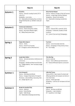


![ik¡p vifBr rhu x| o nks i|] ik¡p izfrosnu] fucU/k& Hkz"Vkpkj] Hkkjr](http://cdn1.abcdocz.com/store/data/001094675_1-29f2b02a82f718abac38e9fa354cfa53-250x500.png)


© Copyright 2026