1. science
2. mathematics
3. algebra

Convergence of two-step Newton methods for
solving nonlinear equations in Banach spaces
Wen Zhou∗
Abstract
In this paper, we consider a family of two-step Newton-like methods for nonlinear equations in Banach spaces. We make an attempt to establish the semilocal
convergence of high-order Newton-like methods under the weak conditions by using recurrence relations. We derive the recurrence relations for the methods, and
then obtain an existence-uniqueness theorem to give the R-order of the methods
and a priori error bounds. Finally, we apply this family of high-order methods to a
simple and typical example of flow in porous media, and show that these methods
are better than Newton’s method.
MSC: 65D10; 65D99
Keywords: Nonlinear equations in Banach spaces; Newton-type method; Recurrence relations; Semilocal convergence.
1
Introduction
We consider the solution of nonlinear equations in Banach spaces given by
F(x) = 0,
(1.1)
where F : Ω ⊆ X → Y is a nonlinear operator on an open convex subset Ω of a Banach
space X with values in a Banach space Y . Such equations include the nonlinear differential equations, the nonlinear integral equations, nonlinear algebraic equations, and so
on.
Iterative methods are often used for solving (1.1). The most well-known iterative
method is Newton’s method [13]
xn+1 = xn − F 0 (xn )−1 F(xn ),
(1.2)
which has quadratic convergence. In order to accelerate the convergence, a family of
third-order methods for scalar case has been presented in [10] and here, we consider its
∗ Department of Foundation Courses, Hubei Vocational Technical College, Xiaogan 432000, Hubei,
China.
1
extension in Banach spaces
xn+1 = xn −
1
Γn F(yn ) + (θ 2 + θ − 1)F(xn ) ,
2
θ
(1.3)
where θ ∈ R, θ 6= 0, Γn = F 0 (xn )−1 , zn = xn − Γn F(xn ) and yn = xn + θ (zn − xn ).
This family of methods requires only one more evaluation of F per iteration than
Newton’s method, but the R-order of convergence is improved to three for sufficient
regular zeros of F. Therefore this family can be more efficient and of practical interest.
The special one (θ = 1) of the family given by (1.3) has been studied in [14], and
it is applied for a basic conservative problem arisen from a nonlinear boundary-value
problem [4]. Another special one (θ = −1) is presented in [11] for solving the single
equation, and then it is successfully used to solve non-symmetric algebraic Riccati
equations arising in transport theory [12].
The convergence of the iterative methods in Banach spaces is often derived using
a majorizing function [7, 19–21]. In [15], the approach of recurrence relation is developed to establish the convergence of Newton’s method, and up to now, it is also successfully used to establish the convergence of some higher-order methods [1,2,5,6,8,9].
In this paper, we shall use recurrence relations to establish the semilocal convergence for the methods given by (1.3) to solve nonlinear equations in Banach space.
We construct the system of recurrence relations for (1.3). We derive the convergence
analysis based on recurrence relations of the methods and obtain the error estimate.
Fluid flow through porous media is a subject of most common interest in hydrology
and petroleum reservoir engineering [3, 16–18], in which various nonlinear differential
equations occur frequently. In this work, we apply the methods given by (1.3) to a
simple and typical example of flow in porous media, and we also present numerical
comparison to Newton’s method.
2
Preliminary results
Definition [13]. Let Π be an iterative process for the nonlinear operator F with
limit point x∗ . The R-order of Π is defined by the quantity
(
∞, if Rq (Π, x∗ ) = 0, ∀q ∈ [1, ∞),
∗
OR (Π, x ) =
inf{q ∈ [1, ∞)|Rq (Π, x∗ ) = 1}, otherwise,
where
(
∗
Rq (Π, x ) =
lim supn→∞ kxn − x∗ k1/n , if q = 1,
n
lim supn→∞ kxn − x∗ k1/q , if q > 1.
If 0 < Rq (Π, x∗ ) < 1 holds for some q ∈ [1, ∞), then the R-order of convergence of
Π is q.
Let an initial approximation x0 ∈ Ω and the nonlinear operator F : Ω ⊂ X → Y be
continuously second-order Fr´echet differentiable where Ω is an open set and X and Y
2
are Banach spaces. We assume that
(C1) kΓ0 F(x0 )k 6 η,
(C2) kΓ0 k 6 β ,
(C3) kF 00 (x)k 6 M, x ∈ Ω,
(C4) kF 00 (x) − F 00 (y)k 6 ω(kx − yk), ∀x, y ∈ Ω, where ω(t) is a non-decreasing
continuous real function for t > 0 and ω(0) > 0,
(C5) there exists a non-decreasing positive real function ϕ ∈ C[0, +∞), with ϕ(t) 6 1
for t ∈ [0, 1], such that ω(ts) 6 ϕ(t)ω(s), for t ∈ [0, 1], s ∈ (0, +∞).
Remark. The conditions (C4) and (C5) are general as they contain the H¨older
continuity of F 00 ; that is, kF 00 (x) − F 00 (y)k 6 Nkx − yk p , ∀x, y ∈ Ω, p ∈ (0, 1]. In
that case, we have ω(s) = Ns p and ϕ(t) = t p that satisfy (C4) and (C5).
R
We denote J = 01 ϕ(t)(1 − t)dt and define the following scalar functions which
will be often used in the later developments. Let
1
g(t) = 1 + t,
2
2
,
h(t) =
2 − 2t − t 2
1
1
1
f (t, u) = th(t) 1 + t
t + Jϕ(g(t))u + Jϕ |θ − 1| + t u.
4
2
2
(2.1)
(2.2)
(2.3)
It is obvious by the definitions that
h(t) =
1
.
1 − tg(t)
Some properties of the functions defined previously are given in the following
lemma.
√
Lemma 1. Let the real functions g, h and f be given in (2.1)-(2.3) and s = 3 − 1
where s is the smallest positive zero of the scalar function g(t)t − 1.
(a) g(t) and h(t) are increasing and g(t) > 1, h(t) > 1 for t ∈ (0, s),
(b) f (t, u) is increasing for t ∈ (0, s), u > 0,
(c) Let ε ∈ (0, 1), then we have g(εt) < g(t), h(εt) < h(t) and f (εt, ε 2 u) < ε 2 f (t, u)
for t ∈ (0, s), u > 0.
Assume that the conditions (C1)-(C5) hold. We now denote η0 = η, β0 = β , a0 =
Mβ η, b0 = β ηω(η) and d0 = h(a0 ) f (a0 , b0 ). Let a0 < s and h(a0 )d0 < 1 where s =
√
3 − 1 is the smallest positive zero of the scalar function g(t)t − 1. We now define the
following sequences for n > 0
ηn+1 = dn ηn ,
(2.4)
βn+1 = h(an )βn ,
(2.5)
an+1 = Mβn+1 ηn+1 ,
(2.6)
3
bn+1 = βn+1 ηn+1 ω(ηn+1 ),
(2.7)
dn+1 = h(an+1 ) f (an+1 , bn+1 ).
(2.8)
From the definitions of an+1 , bn+1 and (2.4)-(2.5), we obtain
an+1 = h(an )dn an ,
(2.9)
bn+1 6 h(an )dn ϕ(dn )bn .
(2.10)
Nextly we shall study some properties of the previous scalar sequences. Later
developments will require the following lemma,
√
Lemma 2. Let the real functions g, h, f be given in (2.1)-(2.3) and s = 3 − 1 where s
is the smallest positive zero of the scalar function g(t)t − 1. If
a0 < s and h(a0 )d0 < 1,
(2.11)
then we have
(a) h(an ) > 1 and dn < 1, ϕ(dn ) 6 1 for n > 0,
(b) the sequences {an }, {bn } and {dn } are decreasing,
(c) g(an )an < 1 and h(an )dn < 1 for n > 0.
Proof. By Lemma 1 and (2.11), h(a0 ) > 1 and d0 < 1 hold. It follows from (2.9)
and (2.10) that a1 < a0 and b1 < b0 . By Lemma 1, we also have h(a1 ) < h(a0 ) and
f (a1 , b1 ) < f (a0 , b0 ). This yields d1 < d0 , ϕ(d1 ) 6 ϕ(d0 ) 6 1 and (b) holds. Based
on these results we obtain g(a1 )a1 < g(a0 )a0 < 1 and h(a1 )d1 < h(a0 )d0 < 1 and (c)
holds. By induction we can derive that items (a),(b) and (c) hold.
Lemma 3. Under the assumptions of Lemma 2. Let γ = h(a0 )d0 , then we have
n
dn 6 λ γ 2 , n > 0,
(2.12)
where λ = 1/h(a0 ), and also for n > 0,
n
n+1 −1
∏ di 6 λ n+1 γ 2
.
(2.13)
i=0
Proof. Since a1 = γa0 , b1 6 h(a0 )d0 ϕ(d0 )b0 6 γb0 , by Lemma 1 we have
1 −1
d1 6 h(γa0 ) f (γa0 , γb0 ) 6 γd0 = γ 2
1
d0 = λ γ 2 .
k
Suppose dk 6 λ γ 2 , k > 1. From Lemma 2, we have ak+1 < ak and h(ak )dk < 1, and
thus
dk+1
6 h(ak ) f (h(ak )dk ak , h(ak )dk ϕ(dk )bk )
6 h(ak ) f (h(ak )dk ak , h(ak )dk bk )
6 h(ak )dk2
k+1
6 h(a0 )λ 2 γ 2
k+1
= λ γ2
.
4
n
Therefore it holds that dn 6 λ γ 2 for n > 0.
By (2.12), we get
n
n
i
∏ di 6 ∏ λ γ 2
i=0
n
i
n+1 −1
= λ n+1 γ ∑i=0 2 = λ n+1 γ 2
, n > 0.
i=0
This shows (2.13) holds. The proof is completed.
Lemma 4. Under the assumptions of Lemma 2. Let γ = h(a0 )d0 and λ = 1/h(a0 ).
The sequence {ηn } satisfies
ηn 6 ηλ n γ 2
n −1
, n > 0.
(2.14)
Hence the sequence {ηn } converges to 0. Moreover, for any n > 0, m > 1, it holds
n+m
∑ ηi 6 ηλ
n 2n −1 1 − λ
γ
m+1 γ 2n (2m +1)
1 − λ γ2
i=n
n
.
(2.15)
Proof. It is easy to obtain
!
n−1
ηn = dn−1 ηn−1 = dn−1 dn−2 ηn−2 = · · · = η
n −1
6 ηλ n γ 2
∏ di
i=0
Because λ < 1 and γ < 1, it follows that ηn → 0 as n → ∞.
Let
n+m
ρ=
i
∑ λ iγ 2 ,
i=n
where n > 0, m > 1. Since
ρ
6
2n
λ nγ + λ γ
!
n+m−1
2n
∑
λ iγ
2i
i=n
n
n
= λ nγ 2 + λ γ 2
n+m
ρ − λ n+m γ 2
,
we can obtain
n
ρ
6
λ nγ 2
n
m +1)
1 − λ m+1 γ 2 (2
n
1 − λ γ2
.
Furthermore, we get
n+m
∑
n
n −1
ηi = ηγ −1 ρ 6 ηλ n γ 2
i=n
Therefore ∑∞
n=0 ηn exists.
3
m +1)
1 − λ m+1 γ 2 (2
n
1 − λ γ2
.
Recurrence relations for the method
The following lemma gives an approximation of the operator F.
5
, n > 0.
Lemma 5. Assume that the nonlinear operator F : Ω ⊂ X → Y be continuously secondorder Fr´echet differentiable where Ω is an open set and X and Y are Banach spaces.
We have
1 00
F(xn+1 ) =
F (xn ) (xn+1 − zn )2 + (xn+1 − zn )(zn − xn ) + (zn − xn )(xn+1 − zn )
2
Z 1
+
F 00 (xn + t(xn+1 − xn )) − F 00 (xn ) (1 − t)dt[(xn+1 − zn )2
0
+(xn+1 − zn )(zn − xn ) + (zn − xn )(xn+1 − zn )]
Z 1
+
F 00 (xn + t(xn+1 − xn )) − F 00 (xn + tθ (zn − xn )) (1 − t)dt
0
(zn − xn )2 ,
(3.1)
where θ ∈ R, θ 6= 0, Γn = F 0 (xn )−1 , zn = xn − Γn F(xn ) and yn = xn + θ (zn − xn ).
Proof. By Taylor expansion, we have
1
1
1
1
−
F(xn ) − 2 F(yn ) + F 00 (xn )(xn+1 − xn )2
F(xn+1 ) =
2
θ
θ
θ
2
Z 1
+
F 00 (xn + t(xn+1 − xn )) − F 00 (xn ) (xn+1 − xn )2 (1 − t)dt,(3.2)
0
and
1
F(yn ) = (1 − θ )F(xn ) + θ 2 F 00 (xn )(zn − xn )2
2
Z 1
F 00 (xn + tθ (zn − xn )) − F 00 (xn ) (zn − xn )2 (1 − t)dt. (3.3)
+θ 2
0
Substituting (3.3) into (3.2), we can obtain (3.1). The real functions g, h, f and the sequences {ηn }, {βn }, {an }, {bn } and {dn } are
defined as the previous section. Let a0 < s, g(a0 ) > |θ |(1 − d0 ) and h(a0 )d0 < 1 where
√
s = 3 − 1 is the smallest positive zero of the scalar function g(t)t − 1.
We denote B(x, r) = {y ∈ X : ky − xk < r} and B(x, r) = {y ∈ X : ky − xk 6 r} in
this paper. In the following, the recurrence relations are derived for the methods given
by (1.3).
For n = 0, the existence of Γ0 implies the existence of y0 . This gives us
kz0 − x0 k = kΓ0 F(x0 )k 6 η0 ,
(3.4)
ky0 − x0 k = |θ |kz0 − x0 k 6 |θ |η0 .
(3.5)
This means that y0 ∈ B(x0 , Rη) where R =
kx1 − z0 k
=
6
g(a0 )
1−d0 .
Consequently, we obtain
1
kΓ0 [(θ − 1)F(x0 ) + F(y0 )]k
θ2
Z 1
0
1
0
kΓ0 k F (x0 + t(y0 − x0 )) − F (x0 ) (y0 − x0 )dt 2
θ
0
6
kΓ0 kkz0 − x0 k2
6
1
Mβ0 η02 .
2
Z 1
tdt
0
(3.6)
6
Therefore we get
1
kx1 − x0 k 6 kx1 − z0 k + kz0 − x0 k 6 η0 + Mβ0 η02 6 g(a0 )η0 .
2
(3.7)
Since the assumption d0 < 1/h(a0 ) < 1, it follows that x1 ∈ B(x0 , Rη).
By a0 < s and g(a0 ) < g(s), we have
kI − Γ0 F 0 (x1 )k
6 kΓ0 kkF 0 (x0 ) − F 0 (x1 )k
6 Mβ0 kx1 − x0 k
6 a0 g(a0 ) < 1.
It follows by the Banach lemma that Γ1 = [F 0 (x1 )]−1 exists and
kΓ1 k 6
β0
= h(a0 )β0 = β1 .
1 − a0 g(a0 )
(3.8)
In consequence, y1 is well defined.
Nextly we consider F(x1 ). By Lemma 5, we can get
Z 1
1
kF(x1 )k 6
M+
ω(tkx1 − x0 k)(1 − t)dt kx1 − z0 k2 + 2kx1 − z0 kkz0 − x0 k
2
0
Z 1
+kz0 − x0 k2
ω(t(kx1 − z0 k + |θ − 1|kz0 − x0 k))(1 − t)dt
0
1
M + Jω(kx1 − x0 k) kx1 − z0 k2 + 2kx1 − z0 kkz0 − x0 k
6
2
+Jkz0 − x0 k2 ω(kx1 − z0 k + |θ − 1|kz0 − x0 k)
1
1
1
M + Jω(g(a0 )η0 ) 1 + a0 a0 η02 + Jω
|θ − 1| + a0 η0 η02
6
2
4
2
1
1
6
M + Jϕ(g(a0 ))ω(η0 ) 1 + a0 a0 η02
2
4
1
+Jϕ |θ − 1| + a0 ω (η0 ) η02 .
(3.9)
2
From (3.8) and (3.9), we have
kz1 − x1 k
= kΓ1 F(x1 )k 6 kΓ1 kkF(x1 )k
6 h(a0 ) f (a0 , b0 )η0
= d0 η0 = η1 .
(3.10)
Because of g(a0 ) > 1, we obtain
ky1 − x0 k
6 ky1 − x1 k + kx1 − x0 k
6
(g(a0 ) + |θ |d0 )η0
< Rη,
which shows y1 ∈ B(x0 , Rη).
7
(3.11)
At the same time, we also have
MkΓ1 kkΓ1 F(x1 )k 6 h(a0 )d0 a0 = a1 ,
(3.12)
kΓ1 kkΓ1 F(x1 )kω(kΓ1 F(x1 )k) 6 h(a0 )d0 ϕ(d0 )b0 = b1 .
(3.13)
By Lemma 2, it follows that η1 < η0 , a1 < a0 < s < 1, b1 < b0 , and d1 < d0 .
Moreover, it holds that g(a1 )a1 < 1 and h(a1 )d1 < 1.
Now we prove the existence of x2 .
kx2 − x1 k 6 g(a1 )η1 .
(3.14)
Since g(t) is increasing for t ∈ (0, s), it holds g(a1 ) < g(a0 ). Therefore, by η1 = d0 η0 ,
we get
kx2 − x0 k
6
kx2 − x1 k + kx1 − x0 k
6
g(a1 )η1 + g(a0 )η0
< g(a0 )(1 + d0 )η0 < Rη.
(3.15)
This shows that x2 is well-defined in B(x0 , Rη).
As a summary result of above process, the system of recurrence relations for (1.3)
given in the next lemma must be satisfied.
Lemma 6. Let the assumptions of Lemma 2 and the conditions (C1)-(C5) hold. Then
the following items are true for all n > 0:
(I) There exists Γn = [F 0 (xn )]−1 and kΓn k 6 βn ,
(II) kΓn F(xn )k 6 ηn ,
(III) MkΓn kkΓn F(xn )k 6 an ,
(IV) kΓn kkΓn F(xn )kω(kΓn F(xn )k) 6 bn ,
(V) kxn+1 − xn k 6 g(an )ηn ,
n+1 2n +1
(VI) xn , yn are well defined in B(x0 , Rη), and kxn+1 − x0 k 6 g(a0 )η 1−λ1−dγ0
where R =
< Rη,
g(a0 )
1−d0 .
Proof. The proof of (I) -(V) follows by using the above-mentioned way and invoking
the induction hypothesis. We only prove (VI). By (V) and by Lemma 4 we obtain
n
kxn+1 − x0 k
6
∑ kxi+1 − xi k
i=0
n
6
∑ g(ai )ηi
i=0
n
6
g(a0 ) ∑ ηi
i=0
n +1
6
1 − λ n+1 γ 2
g(a0 )η
1 − d0
since γ < 1, λ < 1 and λ γ = d0 . This lemma is proved.
8
< Rη,
4
4.1
Semilocal convergence
Convergence theorem
Now we give below a theorem to establish the semilocal convergence of (1.3), the
existence and uniqueness of the solution and the domain in which it is located, along
with a priori error bounds.
Theorem 1. Let X and Y be two Banach spaces and F : Ω ⊆ X → Y be a two times
Fr´echet differentiable on a non-empty open convex subset Ω. Assume that x0 ∈ Ω and
all conditions (C1)-(C5) hold. Let a0 = Mβ η, b0 = β ηω(η) and d0 = h(a0 ) f (a0 , b0 )
√
satisfy a0 < s, h(a0 )d0 < 1 and g(a0 ) > |θ |(1 − d0 ) where s = 3 − 1 is the smallest
positive zero of the scalar function g(t)t − 1 and g, h, f are defined by (2.1)-(2.3) . Let
g(a0 )
B(x0 , Rη) ⊆ Ω where R = 1−d
, then starting from x0 , the sequence {xn } generated by
0
(1.3) converges to a solution x∗ of F(x) with xn , yn , x∗ belong to B(x0 , Rη) and x∗ is the
T
2
− Rη) Ω.
unique solution of F(x) in B(x0 , Mβ
Moreover, a priori error estimate is given by
n −1
kxn − x∗ k 6 g(a0 )ηλ n γ 2
1
n,
1 − λ γ2
(4.1)
where γ = h(a0 )d0 and λ = 1/h(a0 ).
Proof. By Lemma 6, {xn } and {yn } are well-defined in B(x0 , Rη). Now we prove that
{xn } is a Cauchy sequence. Since
n+m−1
kxn+m − xn k
6
∑
kxi+1 − xi k
∑
g(ai )ηi
i=n
n+m−1
6
i=n
n+m−1
6 g(a0 )
∑
ηi
i=n
n
n −1
6 g(a0 )ηλ n γ 2
1 − λ m+1 γ 2 (2
n
1 − λ γ2
m +1)
,
(4.2)
it follows that {xn } is a Cauchy sequence. Thus there exists a x∗ such that limn→∞ xn =
x∗ .
By letting n = 0, m → ∞ in (4.2), we obtain
k x∗ − x0 k6 Rη.
This shows x∗ ∈ B(x0 , Rη).
9
(4.3)
Now we prove that x∗ is a solution of F(x) = 0. It is obtained that
1
1
kF(xn+1 )k 6
M + Jϕ(g(an ))ω(ηn ) 1 + an an ηn2
2
4
1
+Jϕ |θ − 1| + an ω (ηn ) ηn2
2
1
1
6
M + Jϕ(g(a0 ))ω(η0 ) 1 + a0 a0
2
4
1
+ Jϕ |θ − 1| + a0 ω (η0 ) η0 ηn .
2
(4.4)
By letting n → ∞ in (4.4), we obtain kF(xn )k → 0 since ηn → 0. Hence, by the continuity of F in Ω, we obtain F(x∗ ) = 0.
T
2
We prove the uniqueness of x∗ in B(x0 , Mβ
− Rη) Ω. Firstly we can obtain x∗ ∈
T
2
B(x0 , Mβ
− Rη) Ω, since
2
− Rη =
Mβ
2
1
− R η > η > Rη,
a0
a0
2
and then B(x0 , Rη) ⊆ B(x0 , Mβ
− Rη) Ω.
T
2
∗∗
− Rη) Ω. By Taylor theorem, we
Let x be another zero of F(x) in B(x0 , Mβ
have
T
0 = F(x∗∗ ) − F(x∗ ) =
Z 1
F 0 ((1 − t)x∗ + tx∗∗ )dt(x∗∗ − x∗ ).
(4.5)
0
Since
Z 1
0
∗
∗∗
0
kΓ0 k [F ((1 − t)x + tx ) − F (x0 )]dt 0
Z 1
[(1 − t)kx∗ − x0 k + tkx∗∗ − x0 k]dt
Mβ
2
Rη +
− Rη = 1,
2
Mβ
6 Mβ
<
0
(4.6)
it follows by the Banach lemma that 01 F 0 ((1 − t)x∗ + tx∗∗ )dt is invertible and hence
x∗∗ = x∗ .
Finally, by letting m → ∞ in (4.2), we obtain (4.1). This ends the proof. R
4.2
R-order of convergence
We consider the special case that F 00 is of H¨older continuity; that is, ϕ(t) = t p , p ∈
(0, 1]. Similar to Lemmas 3 and 4, we have the following results.
Lemma 7. Under the assumptions of Lemma 2. Let γ = h(a0 )d0 , then
n
dn 6 λ γ (2+p) , n > 0,
10
(4.7)
where λ = 1/h(a0 ), and for n > 0,
n
∏ di 6 λ n+1 γ
(2+p)n+1 −1
1+p
.
(4.8)
i=0
Lemma 8. Under the assumptions of Lemma 2. Let γ = h(a0 )d0 and λ = 1/h(a0 ).
The sequence {ηn } satisfies
ηn 6 ηλ n γ
(2+p)n −1
1+p
, n > 0.
(4.9)
Hence the sequence {ηn } converges to 0. Moreover, for any n > 0, m > 1, it holds
n+m
∑ ηi 6 ηλ n γ
(2+p)n −1
1+p
i=n
(2+p)n ((2+p)m +1)
1+p
1 − λ m+1 γ
n
1 − λ γ (2+p)
.
(4.10)
From the above results, we can derive a priori error estimate
kxn − x∗ k 6 g(a0 )ηλ n γ
(2+p)n −1
1+p
1
n,
1 − λ γ (2+p)
(4.11)
This error estimate indicates that for the case of H¨older continuity of F 00 , the R-order
of (1.3) is 2 + p for p ∈ (0, 1], and especially when F 00 is Lipschitz, the order becomes
three.
5
Numerical results
In this section, we present numerical results to show the performance of the methods given by (1.3). Comparison to Newton’s method is also carried out. Various
nonlinear differential equations need to be treated in fluid flow through porous media [3, 16–18], for example, involving the reactive solute transport with sorption. Here,
we consider a simple and typical example given by
d
dx
−
K
+ x3 = 0, s ∈ (0, 100),
(5.1)
ds
ds
where K is the permeability of porous media and x is the pressure. The boundary
conditions is given by
x(0) = 1, x(100) = 0.
The uniform cell-centered finite difference method [3] is used to discretize the
boundary value problem. Here, we take 100 cells and K = 1. As a result, we obtain a
nonlinear system
F(x) = Ax + G(x) − q,
11
(5.2)
3 )T , q = (2, 0, · · · , 0)T and the mawhere x = (x1 , x2 , · · · , x100 )T , G(x) = (x13 , x23 , · · · , x100
trix A with the size 100 × 100 is given by

3
 −1


A=



−1
2
..
.

−1
..
.
−1
..
.
2
−1



.


−1 
3
We find the solution in Ω = {x ∈ R100 |0 6 xi 6 1, i = 1, · · · , 100}. The norm is
taken as 2-norm. It is easy to find the derivatives of F as
F 0 (x) = A + diag(3xi2 ),
F 00 (x)y = diag(6xi )diag(yi ),
where y ∈ Ω.
The second derivative F 00 satisfies
kF 00 (x)k 6 6 = M,
and
kF 00 (x) − F 00 (y)k 6 6kx − yk,
which x, y ∈ Ω.
We choose [0.5, 0.5, · · · , 0.5]T as the initial approximate solution. Now we apply
the methods given by (1.3) to compute (5.2) and compare it with Newton’s method. We
consider the two cases θ = 1 and θ = −1 for (1.3). All computations are carried out
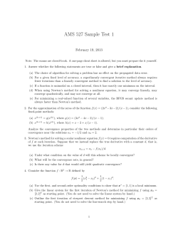
with double arithmetic precision. We plot the numerical solution in Fig. 1, which is
the same for all tested methods. Displayed in Table 1 is the 2-norm of vector functions
(kF(xn )k2 ) at each iterative step.
n
1
2
3
4
5
6
7
8
9
10
11
Table 1. Results of system (5.2) computed by various methods
Newton
Method (1.3) (θ = 1)
Method (1.3) (θ = −1)
0.4129
0.2356
0.2040
0.1090
0.0407
0.0308
0.0314
0.0071
0.0047
0.0090
0.0012
6.5729e-4
0.0025
1.6697e-4
5.1137e-5
6.9121e-4
4.6276e-6
7.4554e-8
1.6143e-4
1.7643e-10
2.0975e-16
1.8675e-5
3.6304e-16
3.2264e-7
9.8612e-11
2.3965e-16
The numerical results demonstrate that the methods given by (1.3) converge faster
than Newton’s method, and the performance of the case θ = −1 for (1.3) is better than
that of θ = 1.
12
1
0.9
0.8
0.7
Solution
0.6
0.5
0.4
0.3
0.2
0.1
0
0
10
20
30
40
50
s
60
70
80
90
100
Figure 1: Computed solution profile.
6
Conclusions
This paper is devoted to a family of high-order two-point Newton-type methods
for solving F(x) = 0 in Banach spaces. We have developed the recurrence relations to
establish the semilocal convergence for the methods. Based on the recurrence relations,
we obtain an existence-uniqueness theorem to establish the R-order of the methods,
which attains to the max order three, and also give a priori error bounds. We apply the
high-order methods to a simple and typical example arisen from flow in porous media,
and numerical examples indicate that these methods are better than Newton’s method.
References
[1] V. Candela, A. Marquina, Recurrence relations for rational cubic methods I: the Halley method, Computing 44 (1990) 169-184.
[2] V. Candela, A. Marquina, Recurrence relations for rational cubic methods II: the Halley method, Computing 45 (1990) 355-367.
[3] C. N. Dawson, H. Kl´ıe, M. F. Wheeler and C. S. Woodward, A parallel, implicit, cell-centered method
for two-phase flow with a preconditioned Newton- Krylov solver, Computational Geosciences, 1 (1997)
215-249.
[4] J.A. Ezquerro, M.A. Hern´andez, M.A. Salanova, A discretization scheme for some conservative problems, J. Comput. Appl. Math. 115 (2000) 181-192.
[5] J.A. Ezquerro, M.A. Hern´andez, Recurrence relations for Chebyshev-type methods, Appl. Math. Optim. 41 (2000) 227-236.
[6] J.A. Ezquerro, M.A. Hern´andez, New iterations of R-order four with reduced computational cost, BIT
Numer Math 49 (2009) 325-342.
[7] J.M. Guti´errez, M.A. Hern´andez, An acceleration of Newton’s method: Super-Halley method, Appl.
Math. Comput., 117 (2001) 223-239.
[8] J.M. Guti´errez, M.A. Hern´andez, Recurrence relations for the Super-Halley method, Comput. Math.
Appl. 7(36) (1998) 1-8.
[9] M.A. Hern´andez, Chebyshev’s approximation algorithms and applications, Comput. Math. Appl. 41
(2001) 433-445.
13
[10] J. Kou, Y. Li, Modified Chebyshevs method free from second derivative for non-linear equations, Appl.
Math. Comput. 187 (2007) 1027-1032.
[11] J. Kou, Y. Li, X. Wang, A modification of Newton method with third-order convergence, Appl. Math.
Comput. 181 (2006) 1106-1111.
[12] Y. Lin, L. Bao, Y. Wei, A modified Newton method for solving non-symmetric algebraic Riccati equations arising in transport theory, IMA Journal of Numerical Analysis, 28(2)(2008) 215-224.
[13] J.M. Ortega, W.C. Rheinboldt, Iterative Solution of Nonlinear Equation in Several Variables, Academic
Press, New York, 1970.
[14] F.A. Potra, V. Pt´ak, Nondiscrete induction and iterative processes, in: Research Notes in Mathematics,
Vol.103, Pitman, Boston, 1984.
[15] L.B. Rall, Computational Solution of Nonlinear Operator Equations, Robert E. Krieger, New York,
1979.
[16] S. Sun and J. Liu, A locally conservative finite element method based on enrichment of the continuous
Galerkin method, SIAM Journal on Scientific Computing, 31(4) (2009) 2528-2548.
[17] S. Sun and M. F. Wheeler, Projections of velocity data for the compatibility with transport, Computer
Methods in Applied Mechanics and Engineering, 195 (2006) 653-673.
[18] S. Sun and M. F. Wheeler, Symmetric and nonsymmetric discontinuous Galerkin methods for reactive
transport in porous media, SIAM Journal on Numerical Analysis, 43(1) (2005) 195-219.
[19] X.H. Wang, Convergence of Newton’s method and uniqueness of the solution of equations in Banach
spaces II, Acta Math. Sin. (English series) 19 (2003) 405-412.
[20] Q. Wu, Y. Zhao, Newton-Kantorovich type convergence theorem for a family of new deformed Chebyshev method, Appl. Math. Comput. 192 (2007) 405-412.
[21] Q. Wu, Y. Zhao, Third-order convergence theorem by using majorizing function for a modified Newton
method in Banach space, Appl. Math. Comput. 175 (2006) 1515-1524.
14