
Health and Air Pollution in New Zealand MAIN REPORT
Health and Air Pollution in New Zealand MAIN REPORT 1 Principal Authors G. Fisher , T. Kjellstrom2, S. Kingham3, S. Hales4, R. Shrestha.5 3 Contributing Authors A. Sturman (Chapter 8), M. Sherman1 (Chapter 8), C. O’Fallon6 (Chapter 10), J.E Cavanagh7 and M. Durand7 (Chapter 10). 1. Endpoint, 2. Health and Environment International Trust, 3. University of Canterbury, 4. Wellington School of Medicine and Health Sciences, 5. Australian National University, 6. Pinnacle Research, 7. Landcare Research. A Research Project Funded by: Health Research Council of New Zealand Ministry for the Environment Ministry of Transport 5 June 2007 This research was funded by the Health Research Council, the Ministry for the Environment and the Ministry of Transport, however, the report may not represent the views of these organisations. Reproduction, adaptation, or issuing of this publication for educational or other non-commercial purposes is authorised without prior permission of the principal authors providing appropriate reference is given. Reproduction, adaptation, or issuing of this publication for resale or other commercial purposes is prohibited without the prior permission of the principal authors. Health and Air Pollution in New Zealand: Final Report ii CONTENTS EXECUTIVE SUMMARY 1. INTRODUCTION........................................................................................................................1 2. 2.1 2.2 3. S1 BACKGROUND ..........................................................................................................................2 Scope 2 Sources and effects of air pollutants 2 2.2.1 Carbon monoxide 3 2.2.2 Nitrogen dioxide 3 2.2.3 Benzene and other hydrocarbons 4 2.2.4 Sulphur dioxide 5 2.2.5 Particulate matter 5 2.2.6 Ozone 7 RELEVANCE TO POLICY .......................................................................................................8 Background 8 Regulatory framework 9 3.2.1 Central government ministries 9 3.2.2 Local government – regional and city councils 11 3.2.3 International agencies 12 3.3 National Environmental Standards – Air Quality 12 3.4 Business sector and private individuals 13 3.5 Summary 14 3.1 3.2 4. OVERSEAS RESEARCH .........................................................................................................15 Scope 15 Air pollution and health effect links 15 4.2.1 Air pollution episodes 15 4.2.2 Epidemiological studies 15 4.2.3 The relationship between exposure duration and effects 16 4.2.4 Effects of exposure from different sources 18 4.3 A more detailed review of studies of the effects of PM10 19 4.3.1 Introduction 19 4.3.2 Time-series studies of particulate matter and mortality 19 4.3.3 Multi-city studies 20 4.3.4 Problems with the GAM model 22 4.3.5 Shape of the dose–response relationship 23 4.3.6 Threshold 24 4.3.7 Effects of particles from different sources 25 4.3.8 Distributed lag models 26 4.3.9 Harvesting (mortality displacement or ‘hastened deaths’) 28 4.4 Update for 2007 based on recent reviews 30 4.5 Summary 31 4.1 4.2 5. NEW ZEALAND BACKGROUND .........................................................................................32 Scope 32 Applicability of overseas research 32 Previous New Zealand studies on air quality and health 34 5.3.1 Epidemiological and clinical studies 34 5.3.2 Health impact and risk assessments 35 5.3.3 The Ministry of Transport health impact assessment, 2002 35 5.3.4 The HAPiNZ Christchurch Pilot Study 36 5.4 Update 37 5.5 Summary 37 5.1 5.2 5.3 Health and Air Pollution in New Zealand: Final Report iii 6. CONFOUNDING FACTORS IN EPIDEMIOLOGICAL STUDIES ...................................38 What is a confounding factor? 38 Potential confounding factors 38 6.2.1 Climate factors 38 6.2.2 Influenza 39 6.3 Adjustments 41 6.3.1 Age, sex and ethnic group 41 6.4 Summary 41 6.1 6.2 7. EPIDEMIOLOGICAL STUDIES AND DOSE−RESPONSE RELATIONSHIPS..............42 Scope of new studies 42 7.1.1 Christchurch 42 7.1.2 Daily time-series analysis 42 7.1.3 Auckland studies 43 7.2 Daily time-series dose−response estimates: Christchurch study 43 7.2.1 Methodology 43 7.2.2 Features of air pollution exposure that influence the health risks 45 7.2.3 Results: mortality 48 7.2.4 Distributed lag analysis and hastened deaths 56 7.2.5 Summary of findings for Christchurch 58 7.3 Spatial variation (first Auckland study) 58 7.3.1 Methodology 59 7.3.2 Potential confounding variables (including climate) 60 7.3.3 Analytical methods 61 7.3.4 Results 61 7.4 Spatial variation (second Auckland study) 62 7.5 Spatial variation (Christchurch study) 67 7.6 Discussion of the new epidemiological studies 68 7.6.1 Dose−response functions 68 7.7 Summary 70 7.1 8. NATIONAL EXPOSURE MODEL .........................................................................................72 Study objectives 72 Study methods 72 What is exposure? 73 Study areas 73 Method 76 8.5.1 Domestic sources 76 8.5.2 Traffic sources 77 8.5.3 Industrial and commercial sources 78 8.5.4 Natural background concentrations 79 8.6 Results and discussion 79 8.6.1 Generated regression equations 79 8.6.2 Estimated pollution concentrations 79 8.7 Model validation 81 8.7.1 Model validation 81 8.7.2 Discussion 83 8.8 Other contaminants 83 8.9 Summary 83 8.1 8.2 8.3 8.4 8.5 9. 9.1 9.2 HEALTH EFFECTS ASSESSMENT ......................................................................................85 Scope 85 Methodology 85 9.2.1 Health impacts of PM10 on mortality 85 9.2.2 Health impacts of PM10 on morbidity 86 9.2.3 Health impacts of CO, NO2 and SO2 87 9.2.4 Cancer risk from benzene 88 9.2.5 Restricted-activity days 88 Health and Air Pollution in New Zealand: Final Report iv Results 9.3.1 Model 9.3.2 Confidence limits 9.3.3 Mortality 9.3.4 Morbidity 9.3.5 Summary 9.3.6 Context 9.4 Summary 9.3 88 88 88 91 92 93 94 95 10. ECONOMIC IMPACT ASSESSMENT ..................................................................................98 10.1 Scope 98 10.2 Methodology 98 10.2.1 Data sources 100 10.2.2 Calculation methods 100 10.3 Discussion 103 10.4 Results 105 10.4.1 Analysis choices 105 10.4.2 Total costs 105 10.4.3 Discussion 106 10.5 Outcome 106 10.6 Summary 108 11. PREVENTIVE POLICY ASSESSMENT..............................................................................109 11.1 Scope 109 11.2 National policy 109 11.3 National environmental standards 109 11.4 Transport emissions issues 110 11.5 Sources of particulate matter from transport 110 11.5.1 Vehicle fuels 110 11.5.2 Petrol engines 114 11.5.3 Diesel engines 115 11.5.4 Hybrid engines 116 11.5.5 Road dust 117 11.5.6 Driving conditions / driver behaviour 118 11.6 Exposure to particulate matter from transport 118 11.6.1 Proximity to roadway 119 11.6.2 In-vehicle exposure 120 11.6.3 Exposure while travelling, by mode 120 11.7 Relationship between particulate matter and other vehicle air emissions 122 11.8 Effect of New Zealand transport interventions on PM emissions 124 11.8.1 The 10 second rule 126 11.8.2 Proposed visual smoke test 126 11.8.3 Accelerated vehicle scrappage programmes 127 11.9 Domestic emissions issues 128 11.9.1 Factors that lead to poor air quality from domestic wood burners 128 11.9.2 Approaches available to reduce domestic wood smoke air pollution 128 11.9.3 Overview of standards for new wood burners 129 11.9.4 Approved wood burners 130 11.9.5 Compliance of approved wood burners 130 11.9.6 Heating system replacement with low emission or zero emission technologies 131 11.9.7 Modifications to wood burners 131 11.9.8 Alternative fuels and add-on devices for wood burners 132 11.9.9 Efficacy of potential mitigation options 133 11.9.10 External influences 133 11.10 Wood burner mitigation programmes 133 11.10.1 Policies 134 11.11 Industrial emissions 134 Health and Air Pollution in New Zealand: Final Report v 11.11.1 Major sources 11.11.2 Minor sources 11.11.3 Discussion 11.12 Summary 12. 134 135 135 135 CONCLUSIONS ......................................................................................................................137 GLOSSARY ........................................................................................................................................138 Disease, outcome and factor measures 138 Risk factors 139 Risk measures 139 Validity vs. bias 141 Other terms 142 Sample selection/allocation procedures 143 General statistical terms 144 Data description 146 Data display 147 Statistical analysis methods 148 Meteorology and modelling 149 Air pollution 151 REFERENCES ...................................................................................................................................153 APPENDICES (GIVEN IN A SEPARATE VOLUME) Appendix 1: Tables of results for each city area Appendix 2: Maps of the city areas covered Health and Air Pollution in New Zealand: Final Report vi Executive Summary Overview The people of New Zealand are exposed to a wide range of health risks through various activities. Many of these are unavoidable, and many are due to personal choice. However, some are due to exposures to contaminants in the environment that can be reduced. This study is concerned with identifying and quantifying the health risks due to people’s exposure to air pollution. For many places, and for much of the time, New Zealand’s air pollution cannot be considered poor by international standards, yet there are still measurable health effects, and there are locations and instances where air quality is poor enough to be of concern. Measures to reduce air pollution and its effect on public health have costs. Effective management and policy therefore needs detailed information on exactly what air pollution occurs and what effects it has. The aim of this Health and Air Pollution in New Zealand (HAPiNZ) study is to explicitly identify the effects of air pollution throughout New Zealand, to link these effects to the various sources of air pollution, and to provide information that will help to formulate effective policy options that lead to real and measurable improvements in the health of New Zealanders. Methodology and scope This study covers the whole of New Zealand. The methodology and scope of the project is large and complex. There are many different sources of air pollution, which are transported around the atmosphere by the weather in complex ways that have a wide range of health effects on the population. Effective policy analysis needs to use accurate information on just which sources have particular effects on particular sectors of the population, in some cases over many years. The study has been funded under a joint initiative from the Health Research Council of New Zealand, the Ministry for the Environment and the Ministry of Transport, with substantial in-kind contributions from Regional Council air quality monitoring programmes. The work has been carried out by a large collaborative group, comprising several organisations and a number of New Zealand’s leading researchers in air pollution, epidemiology, toxicology, environmental management and public health policy. Background A large number of epidemiological studies carried out worldwide have shown associations between ambient air pollution levels and adverse health effects, including increased mortality. The short-term mortality increase in relation to daily levels of particulate matter (PM10 or PM2.5) is approximately 0.5−1% increase per 10 µg/m3 PM10 increase. A variety of statistical methods have been used, and they all come to similar conclusions. The epidemiological analysis demonstrates that the mortality effect of high air pollution lasts longer than the first day of exposure. The resulting long-term mortality increase associated with long-term exposure is substantially higher than the short-term increase. Recent advanced statistical analysis indicates that the mortality increase per 10 µg/m3 PM10 may be as high as 5–10%. The exact biological mechanisms by which air pollution causes increased morbidity and mortality remain to be determined. It would seem that inflammation of the airways is a common pathway for several air pollutants, and that there are direct effects on the cardiovascular system. It is also apparent that some groups within the population are particularly susceptible to the effects of air pollution, including the Health and Air Pollution in New Zealand: Final Report S1 elderly, people with existing respiratory and cardiovascular disease, asthmatics, young children and infants. Another issue that has not yet been resolved is whether PM10 air pollution from different sources causes different levels of health risk. However, the conclusions from several reviews are that PM10 from the main sources of vehicles, wood smoke and industrial sources should be considered of similar toxicity. General results The results obtained from the study are wide-ranging and detailed. All the major sources are included, all the common air pollutants are included, the major effects have been quantified, the economic costs have been assessed, and some typical policy options have been identified and discussed, particularly in relation to transport and domestic heating. The following general results are clear. • The results of previous studies on the effects of air pollution in New Zealand are broadly confirmed, but with greater detail in terms of the location and scale of these effects. In particular, the results are consistent with the 2002 study ‘Health effects due to motor vehicle pollution in New Zealand’, commissioned by the Ministry of Transport (Fisher et al., 2002), and with similar studies conducted overseas. • New epidemiological studies as a part of HAPiNZ carried out in Christchurch and Auckland confirm evidence from overseas studies of short-term effects on mortality, and indicate that the dose−response relationship risk coefficients for longer-term effects are possibly greater than previously thought. • It is estimated that effects occur throughout New Zealand – not just in the main cities. The health impact assessment in the study examines 67 urban areas throughout the country, chosen based on either their size, local activities, and/or monitoring data that shows high levels of air pollution. The study areas comprise 2.7 million people (as of the 2001 census), or 73% of the population of New Zealand. • The greatest effect occurs due to premature mortality associated with long-term exposure to fine particulates from combustion sources. Mortality effects due to carbon monoxide (CO) and various morbidity (non-mortality illness) effects associated with various air pollutants are also identified. • There are adverse effects from air pollution that may not have direct and obvious public health implications, but nevertheless have effects on society. These include restricted-activity days, which can affect large portions of the population on bad, or even moderate, air pollution days. • The most sensitive portions of the population are: (a) older people, particularly over-65s; (b) infants, particularly under-ones; (c) asthmatics and people with bronchitis; (d) people with other respiratory problems; (e) people with other chronic diseases, such as heart disease. • The effects due to various sources have been estimated. These are largely as expected: (a) homeheating solid fuel combustion; (b) industry and commercial activities; and (c) motor vehicle emissions. Some attempt has been made to attribute specific effects to specific sources. The study has included background concentrations (those largely due to natural sources), which allows for more informed policy choices. • Mitigation options are available for new policies and actions at the government, industry and community level. Specific results New epidemiological studies This study has, for the first time, provided detailed epidemiological information on both the short-term and long-term effects on mortality of exposure to urban air pollution in New Zealand. Hourly and daily Health and Air Pollution in New Zealand: Final Report S2 levels of PM10, CO and nitrogen dioxide (NO2) from air monitoring and modelling were used in a timeseries analysis of daily mortality, initially in Christchurch. The results showed that PM10 levels were consistently associated with an increase in daily non-external mortality (excluding injuries and selfinflicted deaths) in the age groups above 65 years of age: approximately 1% increase in mortality for each increase of PM10 by 10 µg/m3. Distributed lag analysis of daily mortality over 40-day periods has indicated that a cumulative effect occurred, leading to greater effects. The results are similar to findings in numerous studies in overseas cities and confirm that mortality is increased by urban air pollution in New Zealand towns and cities. The longer-term effects were studied using modelling of the spatial distribution of air pollution in Auckland (NO2 and PM10) and Christchurch (PM10), estimating annual average exposure in each census area unit within the urban areas, and analysing the association between these exposure estimates and annual mortality adjusted for age, sex, ethnic group, smoking habits and occupational mix. The census area units comprise, on average, groups of 2,300 people, so this analysis has been conducted at a very fine scale (typically overseas studies cover entire cities of several million people agglomerated together). The results indicate higher risks than the short-term time-series studies, which is in line with results from longer-term studies overseas. In Auckland, the non-external mortality increase (averaged for all age groups) for each 10 µg/m3 increase of NO2 was 10% (95% confidence interval: 7–13 %), and for each 10 µg/m3 increase of PM10 it was 6% (95% confidence interval: 1–11%). The risks for mortality from respiratory diseases were the highest. These results support the use of higher risk coefficients in health impact assessments than those produced by short-term time-series studies. The Christchurch and Auckland studies were used to confirm the risk rates appropriate for the rest of New Zealand. Here a 4.3% mortality increase was used for each increase of PM10 by 10 µg/m3 in the preliminary analysis (Fisher et al., 2002). These revised New Zealand findings support the continued use of this risk coefficient for health impact assessments in New Zealand urban areas, although there is growing evidence for the use of a higher risk coefficient (i.e. resulting in potentially greater effects than are reported here). Epidemiology summary It appears from the data presented in this report and the subsequent discussions that the 4.3% increase of mortality for people over age 30 used by Kunzli et al. (2000) for all sources of PM10, while used here, may in future not necessarily be the best available estimate of the dose−response relationship for the purposes of health risk assessments in New Zealand. Taking the recent study by Pope et al. (2002), the HAPiNZ study by Scoggins et al. (2004), the review by Pope & Dockery (2006) and the new results presented in this report into account, it can be concluded that the true figure for annual non-external mortality increase in New Zealand could be in the range 4–8% for each 10 µg/m3 increase of annual average PM10. However, more evidence on any differences in toxicity between vehicle smoke and wood smoke is needed before any modifications of the dose−response relationships are made. As a result, the health risk assessments in this report will be based on the same dose−response coefficient as in the previous assessments, and in Kunzli et al. (2000): 4.3% increase of annual mortality per 10 µg/m3 annual PM10 for all air pollution sources (vehicle, industry and domestic), in the age group above age 30. This makes it possible to compare this new health impact assessment with that produced in the earlier Ministry of Transport report (Fisher et al., 2002). Exposure assessment methodology Another significant component of this study has been the development of a new air pollution exposure model for New Zealand, represented by 67 urban areas (see Table E-1), and covering 73% of the total population. Because the study included many cities that have little or no monitoring, a new method had to Health and Air Pollution in New Zealand: Final Report S3 be established to assess exposure. Full airshed modelling was not possible, again because of the lack of input data, but also because of the resources required to cover 67 areas. Table E-1. 1. 2. 3. 4. 5. 6. 7. 8. 9. 10. 11. 12. 13. 14. 15. 16. 17. 18. 19. 20. 21. 22. 23. 24. 25. 26. 27. 28. 29. 30. 31. 32. 33. Urban areas covered in the study (listed alphabetically) Alexandra Arrowtown Ashburton Auckland Balclutha Blenheim Cambridge Christchurch inner suburbs Christchurch outer suburbs Clevedon Cromwell Dunedin Feilding Geraldine Gisborne Gore Hamilton Hastings Hawera Invercargill Kaiapoi Kaikoura Leamington Levin Lower Hutt Manukau Masterton Matamata Milton Morrinsville Mosgiel Napier Nelson 34. 35. 36. 37. 38. 39. 40. 41. 42. 43. 44. 45. 46. 47. 48. 49. 50. 51. 52. 53. 54. 55. 56. 57. 58. 59. 60. 61. 62. 63. 64. 65. 66. 67. New Plymouth North Shore (Auckland) Oamaru Opotiki Orewa Palmerston North Papakura Paraparaumu Porirua Pukekohe Putaruru Rangiora Reefton Richmond Rotorua Takanini Taupo Tauranga Te Awamutu Te Kuiti Timaru Tokoroa Upper Hutt Waiheke Island Waimate Wainuiomata Waitakere Waiuku Wanganui Wellington Westport Whakatane Whangarei Winton The model has been validated by: (a) comparison with areas where full airshed modelling and previous studies have been carried out (mainly Auckland and Christchurch); and (b) comparison with all PM10 monitoring available (kindly supplied by every Regional Council with a monitoring programme). The model validation shows that realistic exposures have been obtained. The model is based on PM10, but data was also needed on other pollutants that have effects (mainly NO2, CO, and benzene). Thus an additional part of the study has been to establish the relationships between PM10 and these other pollutants. Again the validations undertaken (and related research conducted under the Foundation for Research Science and Technology programme “Keeping New Zealand’s Air Clean”) show this approach to be reasonable. The model developed is not only used for the health assessment made here, but has wider applicability and interest in other sectors to evaluate and manage air pollution. In particular, it provides many Regional Councils with information on air quality in some centres that was not previously available. This information will be used in support of council policies to meet the requirements of the Health and Air Pollution in New Zealand: Final Report S4 National Environmental Standards: Air Quality, which in some cases require aggressive measures to meet the 2013 compliance targets. The results of the exposure analysis for each of the air pollutants considered are given in complete tables in Appendix 1 to the main report. These show that many of these areas experience degraded air quality that would not meet the standards, and this may have serious health effects on their communities. Exposure assessment summary This study has employed a new technique to calculate the exposure to air pollution for 67 city areas in New Zealand. This had to be done because the resources and basic data were not available to make a good assessment based on either monitoring or advanced airshed modelling. All the available PM10 monitoring data, supplied by the Regional Councils, was used in the development and validation of the new model. The data used was basic indicators of activity that results in air pollution – vehicle flow statistics, population density, number of wood burners, location and size of industrial discharges, and an estimate of background concentrations. This data was obtained from standard sources, mainly Statistics New Zealand and the Ministry of Transport, and so the analysis year had to be 2001 – the latest year for which the required input data was available at the time of the major analysis. The methodology has used regression methods to estimate PM10 pollution for all urban areas of New Zealand down to the census area unit level, using these very basic data sources. The values generated accurately predict measured values in those areas where measurements were taken the correlations are similar to those achieved in other similar studies. Indeed, the agreement between the model estimates of annual concentrations and the monitoring of PM10 was remarkable given the variability of air pollution behaviour. This agreement was not perfect (it was not expected to be), and is only applicable to the annual averages required for the study. The results show that high pollution concentrations generally occur in towns with: • colder climates, leading to a greater use of wood burning for heating • easy access to wood as a resource • poor exposure to inhibit pollution dispersion • significant numbers and/or densities of traffic. The higher exposures were found in Nelson, followed by Alexandra and central Christchurch. The results are much as anticipated, and are consistent with more up-to-date monitoring that has been conducted by the councils. However, here the significant advance is that the exposure has been quantified on a nationally consistent basis, and agrees with more advanced analyses in those areas where such analyses have been conducted (e.g. Christchurch and Auckland). The significance of the work is highlighted by the recent acceptance of a paper describing the work in detail in an international peerreviewed journal (Kingham et al., 2007) This research has estimated the contribution of the main sources of air pollution: domestic heating, vehicles, industry and natural background. Health impact assessment – discussion of methods Any assessment of the health effects due to air pollution is extraordinarily complex. For a start, the level of air pollution is highly variable in space and time, and is affected by the weather, by what is being emitted through various activities, and by very location-specific features such as valleys and where people live and work in relation to the sources. Although the concept that ‘dirty air’ is bad for people has been around since ancient times, it is only within the last decade that the mechanisms have started to be identified. Furthermore, a number of largeHealth and Air Pollution in New Zealand: Final Report S5 scale epidemiological studies have shown that effects can occur at quite low levels of pollution, over a wide range of people, due to a number of different exposure scenarios (e.g. which pollutant, over what time period, under which activity). Finally, there is no one measure of ‘air pollution’. It is a common public perception that air pollution is a single thing – most people associate it with visible pollution such as smoke. However, air pollution comprises many components, not all of which are obvious or even detectable by sight or smell by people, and each of which can have different effects, as follows. • Particulates (commonly assessed as PM10 or PM2.5) are very fine particles that can be visible, but are often not obvious. They are associated with increased premature mortality, and exacerbate a number of respiratory and cardiac problems. • Carbon monoxide (CO) is a colourless gas that affects mortality slightly, but exacerbates heart disease and causes drowsiness and learning difficulties. Is strongly correlated with PM10 in cities. • Nitrogen dioxide (NO2) is a slightly brown gas (only detectable when present over large areas) that causes breathing problems, and exacerbates asthma and other respiratory problems. It tends to be correlated with PM10. • Sulphur dioxide (SO2) is a pungent gas that causes sore throat and eyes, and can have an effect on mortality. It is not usually present in hazardous concentrations in New Zealand. • Ozone (O3) is a colourless gas that is present naturally, but causes severe breathing problems in high concentrations. It is not presently a serious problem in New Zealand, with no measured exceedences anywhere. • Benzene is a component of petrol (along with numerous other hydrocarbons) which can lead to cancer. • ‘Air toxics’ refers to a whole range of other toxic compounds, including complex organic chemicals, process chemicals and heavy metals. Little is known about many of these. In summary, while some health effects are well known, others are not, and the state of knowledge is still developing rapidly. A particularly difficult issue that has to be dealt with is the effects of background, or natural, sources. The focus of most air quality research and assessment has been on the three main anthropogenic (humancaused) sources: domestic, vehicle and industrial. Each of these is mainly derived from combustion of some sort, and each is amenable to mitigation policies. However, the implementation of national environmental standards in New Zealand requires a rather detailed knowledge of what causes any particular airshed monitoring result to show exceedence of the standards. The ‘straight-line path’ methodology built into the regulations requires councils to mitigate various sources in order to achieve the standards, but the amount of mitigation required, by source, is variable. A proper analysis requires knowledge of the amount of background air pollution. For instance, if the amount of PM10 due to background sources is a significant fraction of the total, then other sources may need to be mitigated more heavily, because background sources are generally beyond control. In the health effects analysis, the effects of background sources have been explicitly included for this reason. However, it is strongly recommended that extreme caution be applied when attempting to sum the effects into a total effect. It is valid to assign an effect to ‘domestic emissions’, or ‘transport’ or ‘industry’, but it may not be valid to include ‘background’. The research community has not yet resolved the question of whether background sources have the same epidemiological effect as anthropogenic combustion sources. There is some evidence they do not, but on the other hand the background air pollution is included in all the epidemiological studies (after all, it is impossible to get rid of the background). Effects associated with background sources have not been included in the final figures reported, nor in the major conclusions. Health and Air Pollution in New Zealand: Final Report S6 In this study: • domestic sources are emissions from the use of wood and coal in home-heating appliances • vehicle sources are from internal combustion engines on the national roads, using petrol and diesel (they do not include off-road vehicles, trains, ships or aircraft) • industrial sources include all major industries, as well as a factor for smaller commercial activities (such as painting, spraying, wood milling, fish-and-chip shops, etc). Health impact assessment – results The health effects for all the areas studied are summarised in Table E-2. The overall total is included, but it does not include background sources that (a) cannot be mitigated and (b) may well not have the same level of effect as the emissions from the other sources. Table E-2. Effects of air pollution in New Zealand, by source and effect, 2001 (number of cases for the population over 30 years old) Effect Domestic Vehicle Industrial Total 356 414 131 901 70 86 22 178 Bronchitis and related 887 541 116 1,544 Acute respiratory admissions 267 163 35 465 Acute cardiac admissions 137 83 18 238 19 22 6 47 1,105,000 671,000 145,000 1,921,000 Mortality (for PM10, NO2) Mortality (for CO) Cancer Restricted-activity days Table E-2 shows that in the 67 urban areas studied, air pollution is associated with: • 1,079 cases of premature mortality – that is, people dying earlier than they would have if they had not been exposed to air pollution, mostly associated with PM10 (901), but also with CO (178) • 1,544 extra cases of bronchitis and related illnesses • 703 extra hospital admissions for respiratory (465) and cardiac illnesses (238) • 1,921,000 restricted-activity days – that is, days on which people cannot do the things they might otherwise have done if air pollution was not present. The bulk of these effects are associated with particulate pollution (PM10), but there are also effects associated with other pollutants, such as NO2, CO and volatile organic compounds. These results can be put into context by examining how they increase the natural mortality rate. Both natural mortality rates and air pollution rates vary substantially over the country. Natural rates, with a national mean of 6.5 per 1,000 people per year, vary from a low of 5.5 in North Shore City, to a high of 8.0 in Porirua. The air pollution-related mortality rates vary from a low of 0.18 per 1,000 people per year in New Plymouth (low pollution levels due to its very exposed location) to a high of 0.74 in central Christchurch (due to its sheltered meteorology and high rate of wood burner use). The national average increase in the base mortality rate associated with air pollution is 4.8%, ranging from 2.9% in New Plymouth to 11.8% in Christchurch. This result implies that, nationally, 1 in 20 people (4.8%) die earlier than they would have because of air pollution. In Christchurch (and some other South Island towns with very high pollution levels) this could be as high as 1 in 9 people. This result should not be interpreted too dramatically, although it certainly indicates a situation to be avoided by reducing air pollution. The concept of premature mortality means that some of these people Health and Air Pollution in New Zealand: Final Report S7 may be dying a matter of days or weeks earlier than they would have otherwise. But it also means that they may be dying months or years earlier, resulting in high economic and social costs. Health effects summary The health impact assessments shown here are based on exposures derived from modelling and validated against monitoring and published dose−response relationships. The health effects have been calculated with two overall constraining factors. 1. The study has been prioritised and based on the factors known to be associated with the greatest health effects – mainly the longer-term exposures, and the exposure to PM10. Effects due to some other pollutants have been analysed (e.g. CO, SO2, NO2, and benzene), but these show diminishing effects relative to annual PM10. The CO effects have been included because they are non-trivial. Benzene effects are also included, but these are very small relative to PM10 and CO. Others (such as SO2 and other types of air pollution) are negligible on the national scale relative to the ones included. Effects associated with NO2 are non-trivial, but these are intimately associated with PM10 effects and are not able to be identified separately. They are assumed to be included in the PM10 effects – to avoid double counting of effects – but there is growing evidence that there may be separate and independent effects associated with NO2 exposure, especially in children. 2. The dose−response relationships used for analysing the health effects are conservatively chosen from those used for a number of years in the international literature, and used by many other countries, including the USA, the European Union and Australia. There is growing evidence that some of these dose−response relationships have been underestimated, or could be applied in a more sophisticated way. However, the evidence is not yet strong enough to justify these newer methodologies in a study of this nature. The implication is that the results given here are conservative: it is likely that once new dose−response relationships are confirmed, these will show a great health burden due to atmospheric pollution in New Zealand. The results show a number of relevant features (relevant to the 2001 population). • The greatest health effect for all pollutants is associated with long-term exposure to elevated concentrations of PM10 (increased premature mortality in over 30-year olds of 901 cases per year). • Effects can occur at relatively low levels, and thus can occur to some extent in every city studied. • Effects could also be due to background levels (i.e. PM10 that comes from natural sources such as wind-blown dust and even sea spray). These effects have been included in the analysis because mitigation policy options need to account for them, but they should be viewed with caution because the epidemiology on this topic is incomplete. • Effects associated with CO also show a significant level of premature mortality (178 cases per year) and illness (2,247 extra hospital admissions for respiratory and cardiac disease per year). • These air pollution effects include premature mortality, respiratory illness, cardiac illness and restricted-activity days (1,921,000 days per year). • The overall burden of health effects is borne by the larger urban areas, principally because of the size of the populations. These include all the greater Auckland region cities, Christchurch, greater Wellington, Hamilton, Tauranga and Dunedin. Although air pollution levels in many South Island cities are higher than in the major centres, the total number of cases of health effects is lower simply because the populations are lower. However, the proportion of the population affected will be higher in those areas with higher amounts of air pollution. • The population within the study areas has grown by 17% from 2.73 million in 2001 to 3.20 million in 20071, so it is reasonable to assume that the current total health costs are also 17% greater for most 1 See http://www.stats.govt.nz Health and Air Pollution in New Zealand: Final Report S8 of the figures derived above (although due to differences in the rates of population growth in various areas, this increase cannot be applied equally in all areas). • Finally, a comment is required on the nature of these epidemiological results. They are long-term statistics, designed to give an indication of the effects, rather than to be a specific predictor for a particular city in a particular year. For instance, the assessment shows that there is one additional case of premature mortality in Arrowtown due to air pollution in that town. This does not mean that one extra identifiable person will die each year in Arrowtown from air pollution (for the population of around 1,600 there would be on average of 13 people dying from natural causes). It does mean that over a period of several years, taking account of the statistical variation in deaths, that on average one person a year will have died earlier than they would have otherwise because of the occurrence of air pollution. These health effects results are complex to calculate and difficult to interpret. This executive summary, along with more detailed results in the appendices, has attempted to give a quantified indication of the total effects of air pollution in New Zealand on the health of its citizens. Economic impact assessment The costs of air pollution effects can be estimated using the new statistics from this study, previous research in New Zealand, and results from overseas studies adjusted for New Zealand conditions. Table E-3 gives a summary of the specific health effects used, and their cost per case. These are not personal costs, but costs to the New Zealand health system and economy – the external costs of air pollution. Table E-3. Estimated costs of specific health effects used in the analysis Effect Cost per case Mortality $750,000 Cancer $750,000 Chronic bronchitis $75,000 Admission (cardiovascular) $3,675 Admission (respiratory) $2,700 Restricted-activity day $92 These figures have a degree of subjectivity, and are estimates only. There is no international, or even national, agreement on how to apply economic analysis, and the values used in various countries can differ widely. For instance, the cost of mortality is argued to be as low as $50,000 to as high as $6,000,000. The figures used here are reasonably conservative estimates, calculated for New Zealand circumstances. Different studies may apply different costs. There are some effects that are not studied, nor explicitly costed, mainly because the research results are not available. These include asthma cases, short-term effects and toxic effects. Similarly, some effects will incur additional costs that are difficult to quantify, including costs of extra doctor’s visits and medication, lower-level effects due to mild but perhaps widespread effects due to drowsiness, headaches, loss of attention and quality of life that may not be included in the restricted-activity day analysis. Finally, the general economic effect of perceptions of ‘poor air quality’ on tourism and recreation are not negligible, but are beyond the scope of this study. The total costs of health effects of air pollution can be estimated from the health effects and the cost per case of those effects. These are shown in Table E-4. By far the largest component of the ‘economic health burden’ is the loss of life-years as a result of premature mortality, followed by restricted-activity days and then chronic bronchitis. Health and Air Pollution in New Zealand: Final Report S9 Table E-4. Annual costs ($million) of air pollution in New Zealand, by source and effect Effect Domestic Mortality (due to PM10, NO2) Vehicle Industrial Total 267.0 310.5 98.3 675.8 Mortality (due to CO) 52.5 64.5 16.5 133.5 Bronchitis and related 66.5 40.6 8.7 115.8 1.2 0.7 0.2 2.1 14.3 16.5 4.5 35.3 Restricted-activity days 101.7 61.7 13.3 176.7 Total 503.2 494.6 141.5 1,139.2 Respiratory/cardiac admissions Cancer When considered across the 2.7 million people in the study areas, these amount to the following costs per person per year: • total effects: $421 per person per year • effects associated with domestic emissions: $186 per person per year • effects associated with vehicle emissions: $165 per person per year • effects associated with industrial emissions: $70 per person per year. Although background and natural sources of air pollution (such as wind blown dust) have been included in the detailed analysis, they are not included in this cost summary. Health costs summary Not all potential costs have been included. For instance, indirect costs, such as doctor’s visits and increased use of medicine, have not been included. There is very little data on these factors, although they are not expected to be insignificant. The total costs of air pollution in New Zealand are in the order of at least $1,139 million per year, based on 2001 statistics. Since the population within the study areas has grown by 17% from 2.73 million in 2001 to 3.20 million in 20072, it is reasonable to assume that the current total costs are also of the order of 17% greater, at $1,333 million. Policy options A number of policy options for reducing emissions, and hence reducing health effects, have been discussed. This discussion is far from comprehensive, since new policies are being continually proposed and the environment in which they operate is constantly changing. However, the results of the study do give a quantified indication − at the level of individual cities and towns, as well as nationally − of the scale of the mitigation policy actions required. During the time that this study has been conducted there has been a great deal of development in the transport policy arena. This has included the introduction of new fuel specifications (significantly reducing the emissions of sulphur and benzene since 2001), the continuing implementation of new emissions standards for vehicles, and a series of public information and education campaigns. The overall result has no doubt been a reduction in air pollution due to vehicle emissions, although this has not been fully quantified here. 2 See: http://www.stats.govt.nz Health and Air Pollution in New Zealand: Final Report S10 Domestic policy options have much more of a local focus – what may be highly relevant for one council may be quite inappropriate for another. In addition, the assessment of domestic heating emissions is currently the subject of active research and assessment by both the Ministry for the Environment and many councils. The importance of reducing domestic heating emissions is accepted by all branches of central and local government, and descriptions of the work being conducted in various programmes exceeds what is possible to cover here. However, a fuller discussion has been developed on some of the reduction methods being applied. When it comes to industrial emissions, one aspect arising from the research has been that, contrary to common public perception, industries do not contribute heavily to the burden of public health associated with air pollution (of the order of 15% nationally, only exceeding this in Auckland City and Manukau, with most regions lower than 1%). They do, of course, in some areas, and the local regulating council is well aware of these in every instance. Without going into great and specific detail, there is little value that can be added beyond what councils already enact. Despite some gaps in the comprehensiveness of the policy options, and some of them being outdated, the information produced by this study does give detailed quantitative information on the contributions from various air pollution sources throughout 67 key urban areas in New Zealand that will be valuable in assessing policy options. Health and Air Pollution in New Zealand: Final Report S11 Acknowledgements The Health Research Council of New Zealand, Ministry for the Environment and Ministry of Transport funded the Health and Air Pollution in New Zealand (HAPiNZ) project through the Environmental Health Joint Research Portfolio. The authors would also like to acknowledge the support of the Ministry of Health, the Auckland Regional Council, Environment Canterbury, and the other regional councils and unitary authorities that have freely supplied their monitoring data for this study. Auckland Regional Council (Kevin Mahon) also helped to update the current state of knowledge at the time of publication. The project involved collaboration with the following named scientists. Some individual research elements of HAPiNZ have been or will be published in other forms. This report primarily covers the health impact assessment and its input data. Contributing scientists (in alphabetical order) Name Institution Dr Jo-Anne Cavanagh Dr Tom Clarkson Dr Janine Clemons Philip Donnelly Dr Michael Durand Dr Charlie Eason Dr Michael Epton Gavin Fisher Dr Neil Gimson Dr Simon Hales Clive Heydenrych Dr Simon Kingham Prof. Tord Kjellstrom Sue McLeod Des O’Dea Carolyn O’Fallon Dr Jamie Pearce Amanda Scoggins Rupendra Shrestha Dr Rachel Spronken-Smith Prof. Andy Sturman Dr Ian Town Dr Louis Tremblay Karen Trout Dr Jeff Wilson Emily Wilton Prof. Alistair Woodward Dr Peyman Zawar-Rewa Landcare Research National Institute of Water and Atmospheric Research (NIWA) Landcare Research Private Consultant Landcare Research Landcare Research Christchurch School of Medicine and Health Sciences NIWA/Endpoint National Institute of Water and Atmospheric Research (NIWA) Wellington School of Medicine and Health Sciences National Institute of Water and Atmospheric Research (NIWA) University of Canterbury Health and Environment Trust University of Canterbury Wellington School of Medicine and Health Sciences Pinnacle Research University of Canterbury National Institute of Water and Atmospheric Research (NIWA) Australian National University University of Canterbury University of Canterbury Christchurch School of Medicine and Health Sciences Landcare Research Landcare Research University of Canterbury Environet Wellington School of Medicine and Health Sciences University of Canterbury (Note: some of these authors have changed affiliation. This list is correct at the time of their contribution.) Health and Air Pollution in New Zealand: Final Report S12 1. Introduction All over the world concern is growing over the health effects of emissions from transport, industry, domestic and other human activities. In New Zealand a 2002 study commissioned by the Ministry of Transport estimated that approximately 400 people aged 30 and over die prematurely each year from exposure to PM10 particulates from motor vehicle emissions. It also estimates that an additional 570 people of the same group die prematurely each year from air pollution derived from other sources (Fisher et al., 2002). As a result of these preliminary findings, the Health Research Council of New Zealand, Ministry for the Environment and Ministry of Transport have commissioned a national ambient air quality management project, Health and Air Pollution in New Zealand (HAPiNZ), to better define the problem for New Zealanders. The major purpose of the project is to determine the environmental, health, social and economic costs of air pollution from all sources in New Zealand. The study is supported by the Ministry of Health, the Auckland Regional Council and Environment Canterbury. Other regional councils, authorities and communities of interest are also involved. PARTNERS R E S E A R C H P R O V ID E R S H e a lth R e s e a rch C o u n c il M in is try o f T ra n sp o rt $$$ M in is try fo r th e E n viro n m e n t A u c k lan d R e g io n a l C o u n c il E n viro n m e n t C a n te rb u ry M in is try o f H e a lth In K in d S u p p o rt N IW A U n ivers ity o f C a n terb u ry C h ristc h u rc h S O M & H ea lth S c ie n c e s W e llin g to n S O M & H e a lth S c ie n c e s A u s tra lian N a tio n a l U n ive rsity L a n d ca re R e se a rc h E n viro n e t P riva te c o n su lta n ts O th e r R e g io n a l C o u n cil, U n ita ry a u th o ritie s , & C o m m u n itie s o f In te re s t e .g . m ed ia , p u b lic Figure 1-1. HAPiNZ collaboration The research has evaluated the effects of specific source categories of emissions from vehicles (including private petrol cars, diesel cars and diesel trucks), industry, domestic and total sources in most urban areas of New Zealand. Source contributions for the following pollutants have been characterised for each defined area: PM10, nitrogen dioxide (NO2), carbon monoxide (CO) and benzene. Ozone (O3) and sulphur dioxide (SO2) were considered because they do have health effects and are covered by standards, but their levels are relatively low in New Zealand and their contribution to the total health effects is very minor compared to the other pollutants. Creating effective, evidence-based policy requires linking health and economic endpoints back to the sources, so that preventive policy options and recommendations can be tailored to address emissions sources in order of their contribution to the air pollution problem. The research has five interconnected components: • • • • • air quality, meteorology and emissions data analysis epidemiological studies of health effects in New Zealand cities air pollution exposure assessment health impact assessment preventative policy options discussion. This report presents the results of the final study covering all of New Zealand. It follows the publication of the Pilot Study on Christchurch, released in November 2005 (Fisher et al., 2005b). Health and Air Pollution in New Zealand: Final Report 1 2. Background 2.1 Scope The purpose of this section is to provide a brief background on the relationship between air pollution and health concerns, and the broad nature of the health effects. 2.2 Sources and effects of air pollutants Urban air pollution is increasingly the result of the combustion of fossil fuels (coal, oil, petrol, diesel, natural gas) for transport, power generation and other human activities. Biomass (wood, agricultural waste) is another important source of air pollution. The infamous London Smog episode during December 1952, caused by intensive coal burning in stagnant weather conditions over several days, led to SO2 and smoke reaching several thousands of micrograms per cubic metre (µg/m3). This resulted in an estimated excess death toll of over 4,000 people. This event and others led to effective actions during the 1950s to 1970s to reduce air pollution, such as requiring emissions controls on industry, power stations and cars, starting as early as 1966. Even so, epidemiological studies through the 1980s till now are finding effects at very low levels of exposure and at levels below existing health guidelines. In July 2004 the New Zealand Government approved national environmental standards aimed at improving air quality and controlling emissions. Table 2-1 shows the maximum level for the amount of CO, NO2, ozone, fine particles (PM10), and SO2 according to the air quality standards. Table 2-1. New Zealand National Environmental Standards Contaminant Threshold concentration Averaging period Permissible excess (in 12 months) Carbon monoxide 10 mg/m3 Running 8-hour 1 x 8-hour period Nitrogen dioxide 200 µg/m3 1-hour mean 9 hours 3 1-hour mean Not to be exceeded Ozone Particulate (PM10) Sulphur dioxide 150 µg/m 50 µg/m 3 24-hour mean 1 x 24-hour period 3 1-hour mean 9 hours 3 1-hour mean Not to be exceeded 350 µg/m 570 µg/m The major sources that emit pollutants include mobile (petrol and diesel cars and trucks), domestic (e.g. wood- and coal-burning heating), industrial (coal or heavy oil power stations) and biogenic or natural (e.g. dust, sea salt) sources. For the purposes of this study, the definitions of the major sources are relatively simple (since data availability on the details of all sources is poor in many areas). • Domestic – all solid-fuel heating appliances (mainly wood, but also some using coal), as identified in the 2001 census. An average emissions rate is assumed. • Vehicle – all vehicles using the national roads, according to the Ministry of Transport survey information for 2001. Off-road vehicles, ships, trains and aircraft are not included. • Industrial – all large dischargers (more than 10 kg per day of PM10 on average, from regional council air discharge consents), as well as an area-based estimate for smaller industries. Health and Air Pollution in New Zealand: Final Report 2 • Background – a factor that includes all other relevant sources such as dust, sea salt, pollen, agricultural burning, etc. This is an estimate because almost no data is available on the nature of these sources. Although particulates (such as PM10 and PM2.5) are most commonly associated with health effects, other studies also link these effects to CO, NO2, SO2, ozone and hydrocarbons. The types and concentrations of pollutants in the ambient air vary greatly from location to location, with time of day and with season. Because these pollutants occur together and are often closely correlated, it has been difficult to clearly identify the effects of single pollutants, or potentially damaging combinations of them. The major pollutants that can produce health effects are the gases CO, nitrogen oxides (NOx), volatile organic compounds and SO2, as well as solid particulate matter (now commonly referred to as particles). Other gases (such as ozone) and particles (sulphates and nitrates) can form in the atmosphere from reactions involving some of these primary emissions. The health effects of CO, NO2, ozone, particles and SO2 have been reported in a number of reviews (e.g. Denison et al., 2000a) and the following is a brief summary of that information. It should be pointed out from the start that air pollution caused by the combustion of fossil fuels or biomass always contains a mixture of several of the pollutants mentioned here, and that epidemiological studies should be interpreted with this in mind. The types of health effects that have been reported as an outcome of exposure to the main air pollutants are briefly mentioned below. Further details of the published evidence about health effects of the air pollutants are presented in section 4 of this report. The focus is on particulate matter, because a number of reviews have concluded that this may be the most problematic pollutant concerning health effects. 2.2.1 Carbon monoxide CO is a colourless, odourless gas formed as a result of incomplete combustion of carbon-containing fuels, including wood, coal, petrol and diesel. CO is readily absorbed from the lungs into the blood stream, which then reacts with haemoglobin molecules in the blood to form carboxyhaemoglobin. This reduces the oxygen-carrying capacity of blood, which in turn impairs oxygen release into tissue and adversely affects sensitive organs such as the brain and heart (Bascom et al., 1996). Motor vehicles are the predominant sources of CO in most urban areas, although domestic heating emissions also contribute. In general there has been a decline in CO concentrations, which reflects the efficacy of emissions control systems on newer vehicles. However, as a consequence of the age of the vehicle fleet, and heavy use of solid fuels in winter for domestic heating, New Zealand has relatively high urban air concentrations of CO. It has been reported that in 2001 nearly 50% of the New Zealand car fleet was more than 10 years old, and only 20% is less than five years old (Ministry of Economic Development, 2001). In addition there are over 500,000 solid-fuel heaters in use, with a significant number of these more than 10 years old with potentially high levels of CO and other air pollution emissions. Long-standing international (and New Zealand) air quality guidelines/standards for CO are based on keeping the carboxyhaemoglobin concentration in blood below a level of 2.5%, in order to protect people from an increased risk of heart attacks. However, there is emerging research that indicates adverse health effects at carboxyhaemoglobin levels less than 2.5% (Morris & Naumova, 1998). This new information is especially relevant to New Zealand, because of the relatively high urban air concentrations of CO. 2.2.2 Nitrogen dioxide Oxides of nitrogen (NOx) (primarily nitric oxide and lesser quantities of NO2) are gases formed by the oxidation of nitrogen in air at high combustion temperatures. Nitric oxide is oxidised to NO2 in ambient air, which has a major role in atmospheric reactions that are associated with the formation of photochemical oxidants (such as ozone) and particles (such as nitrates). NO2 is also a serious air pollutant in its own right. It contributes both to morbidity and mortality, especially in susceptible groups such as young children, asthmatics, and those with chronic bronchitis and related conditions (Morris & Health and Air Pollution in New Zealand: Final Report 3 Naumova, 1998). One study has also shown that exposure during very early childhood can increase the risk of development of asthma induced by other allergens in the home (Ponsonby et al., 2000). NO2 appears to exert its effects directly on the lung, leading to an inflammatory reaction on the surfaces of the lung (Streeton, 1997). Increased lung cancer incidence has also been reported in a large casecontrol study (Nyberg et al., 2000), but NO2 was primarily used as an indicator of air pollution exposure from vehicle emissions, and so other air pollutants from vehicles may have been the cause of the cancers. Motor vehicles are usually the major source of nitrogen oxides in urban areas, although the combustion of fossil fuels from stationary sources (heating, power generation) is also a major source of anthropogenic emissions of nitric oxide. Indoor concentrations of nitrogen oxides typically exceed those existing outside when unvented combustion appliances are used for cooking and heating (e.g. unflued gas heaters). Air quality guidelines/standards for NO2 are set to minimise the occurrence of changes in lung function in susceptible groups. The lowest observed effect level in asthmatics for short-term exposures to NO2 is about 400 µg/m3. Although less data is available, there is increasing evidence that longer-term exposure to about 80 µg/m3 during early and middle childhood can lead to the development of recurrent upper and lower respiratory tract symptoms. A safety factor of 2 is usually applied to those lowest observed effect levels, giving air quality standards for NO2 of 200 µg/m3, 1-hour average (WHO, 2006). 2.2.3 Benzene and other hydrocarbons Volatile organic compounds (VOCs) are a range of hydrocarbons, the most important of which are benzene, toluene, xylene, 1,3-butadiene, polycyclic aromatic hydrocarbons (PAHs), formaldehyde and acetaldehyde. Some of these chemicals are included in the ‘air toxics’ category of pollutants. The potential health impacts of these include carcinogenic and non-carcinogenic effects. Benzene and PAHs are definitely carcinogenic, 1,3-butadiene and formaldehyde are probably carcinogenic, and acetaldehyde is possibly carcinogenic. Non-carcinogenic effects of toluene and xylene include damage to the central nervous system and skin irritation. Heavier VOCs are also responsible for much of the odour associated with diesel exhaust emissions. Motor vehicles are the predominant sources of VOCs in urban areas. Benzene, toluene, xylene and 1,3butadiene are all largely associated with petrol vehicle emissions. The first three result from the benzene and aromatics contents of petrol, and 1,3-butadiene results from the olefins content. Evaporative emissions, as well as exhaust emissions, can also be significant, especially for benzene. Motor vehicles are major sources of formaldehyde and acetaldehyde. These compounds are very reactive and are important in atmospheric reactions, being products of most photochemical reactions. PAHs arise from the incomplete combustion of fuels, including diesel. The most important of the VOCs in the New Zealand context is benzene. The maximum allowable level of benzene in petrol was 3% by volume, but this has been decreasing and was reduced to 1% in 2006. Health effects data and guidelines/standards for hazardous air pollutants have been reported elsewhere (Chiodo & Rolfe, 2000), and include recommended air quality guidelines for benzene of 10 µg/m3 (now) and 3.6 µg/m3 by 2010 (when the benzene content of petrol is reduced), both guidelines being annual average concentrations (Ministry for the Environment & Ministry of Health, 2002). Cancer risks are assessed using inhalation unit risk (IUR). Inhalation unit risks are defined as the individual lifetime excess risk due to a chronic lifetime exposure to one unit of pollutant concentration. Estimates generally assume a no-threshold, low-dose linearity. Based on the WHO (2000) Air Quality Guidelines for Europe, the excess lifetime risk of cancer (leukaemia) at an air concentration of 1 µg/m3 is 6 x 10⁻⁶. This figure was derived from the geometric mean of the range of the calculated unit risk per µg/m3 based on updated results from the Pliofilm cohort study of 4.4 x 10⁻⁶ to 7.5 x 10⁻⁶ (WHO, 2000). The 1987 WHO air quality guideline for Europe gave the unit risk as 4 x 10⁻⁶. The US EPA estimates a range for unit risks from 2.2 x 10⁻⁶ to 7.8 x 10⁻⁶ for an increase in the lifetime risk of an individual who is exposed to 1 µg/m3 of benzene air. Health and Air Pollution in New Zealand: Final Report 4 Benzene and other toxic levels have been measured previously in New Zealand in a number of studies commissioned by the Ministry of Health (Stevenson & Narsey, 1998). The most recent study surveyed benzene and other toxic organic compounds in air from July 1996 to May 1999 in Auckland, Hamilton, Christchurch and Dunedin. The results suggested an additional lifetime leukaemia risk for New Zealand benzene exposures (excluding exposures from active smoking and from evaporative vehicle emissions from indoor garages) in the range of 6 x 10⁻⁶ to 6 x 10⁻⁵. If the whole population were exposed to these levels of risk, they would correspond to between 0.3 and 3 additional leukaemia deaths every year (Stevenson & Narsey, 1999b). 2.2.4 Sulphur dioxide Sulphur oxides (primarily SO2 and lesser quantities of sulphur trioxide) are gases formed by the oxidation of sulphur contaminants in fuel on combustion. SO2 is a potent respiratory irritant, and has been associated with increased hospital admissions for respiratory and cardiovascular disease (Bascom et al., 1996), as well as mortality (Katsouyanni et al., 1997). Asthmatics are a particularly susceptible group. Although SO2 concentrations in New Zealand are relatively low, and motor vehicles are minor contributors to ambient SO2, the measured levels in Auckland (for example) showed an increase in recent years, after many years of decline, as a result of the increasing number of diesel vehicles (and the historically relatively high sulphur content of diesel in New Zealand). However, this trend is now reversing, as a result of the fuel specification reviews in 2005 whereby the maximum sulphur content of fuels has been reduced. For instance, in the 1990s the measured sulphur levels in diesel fuel were 2,500−3,000 ppm. The standard moved to 500 ppm, and is now 50 ppm, with the expectation that it will become lower still to be in line with standards in Europe, the USA and Japan. Preliminary unpublished work suggests that this improvement in fuel specifications will have a significant effect in reducing secondary PM10 concentrations in some cities, resulting in lower health effects. SO2 is also emitted from the combustion of coal, but this does not occur much in cities, and the monitored rates of SO2 are well below the health-based guidelines in all urban areas where monitoring has been conducted. Elevated concentrations (but still below the guidelines) do occur, but only within a few kilometres of major users, and very few people are exposed to these. Sulphur oxides from fuel combustion are further oxidised to solid sulphates, to a certain extent within the engine and completely in the atmosphere. The former inhibits the performance of exhaust emission control equipment for nitrogen oxides and particles, and this is a major reason why the sulphur contents of petrol and diesel have been reduced internationally. It is an unfortunate reality that unless the sulphur content of diesel is less than about 120 ppm, vehicles with advanced emission control systems are actually net producers of additional fine particles because of oxidation of the sulphur oxides to sulphates. With the recent changes to New Zealand fuel specifications this is no longer an issue in this country. There appears to be a threshold concentration for adverse effects in asthmatics from short-term exposures to SO2 at a concentration of 570 µg/m3 for 15 minutes (Streeton, 1997). Ambient air standards are based on this figure; for example, the standard for New Zealand is 350 µg/m3 1-hour average, with ambient guidelines of 120 µg/m3 for the 24-hour average. Note that the WHO (2005) is recommending that this 24-hour guideline be reduced to 20 µg/m3, but as of May 2007 no specific changes have been made to New Zealand’s standards or guidelines. 2.2.5 Particulate matter Evidence from epidemiological studies consistently points to associations between short-term exposure to ambient PM and adverse health effects, even at the low levels commonly encountered in developed countries. Primary particulates are emitted directly from sources such as motor vehicles or wood fires and secondary particles are formed through atmospheric reactions of SO2, nitrogen oxides, and certain organic compounds. Most studies of health endpoints have used ambient PM10 mass concentrations and/or other ambient PM indicators such as PM2.5, black smoke, coefficient of haze, total suspended Health and Air Pollution in New Zealand: Final Report 5 particles, aldehydes (COH) or sulphate. A distinction is made between PM10 (‘thoracic’ particles smaller than 10 µm in diameter which can penetrate into the lower respiratory system), PM2.5 (‘respirable’ or fine particles smaller than 2.5 µm that can penetrate into the gas-exchange region of the lung), and ultrafine particles smaller than 100 nm, which contribute little to particle mass but which are the most abundant and offer a very large surface area, with increasing degrees of lung penetration (Brunekreef & Holgate, 2002). The largest particles (coarse fraction, 2.5–10 um) are mechanically produced by the attrition of larger particles. Fine (small) particles (< 2.5 µm) are largely formed from gases, and the smallest (< 0.1 µm, ultra-fine) are formed by nucleation resulting from condensation or chemical reactions that form new particles. The most recent studies show that, in general, PM2.5 is a better predictor of health effects than PM10 and that it is probably the finer particles causing greater effects, owing to their ability to accumulate and reach the lower regions of the respiratory system. Particles from diesel emissions are possibly having greater effects than those from other sources. Evidence is also emerging that constituents of PM2.5, such as sulphates and strongly acidic particles, are sometimes better predictors of health effects than PM2.5. Many studies have related day-to-day variations in PM to day-to-day variations in health parameters. Acute effects have included increased daily mortality, increased rates of hospital admissions due to the exacerbation of respiratory disease, increased use of bronchodilator medicaments, increased prevalence of cough, and a reduction of peak flow in lung function tests. Although these quantitative estimates of effects of PM10 are generally consistent, there is no apparent threshold concentration below which no effects occur. As a result, the WHO Air Quality Guidelines do not recommend a specific concentration as the ‘health-based maximum’ for particles, but has instead expressed the guideline in the form of dose−response relationships for different health effects (WHO, 2000). Very recently, the WHO published new guidelines that recommend defined limits for many air pollutants (WHO, 2006). The New Zealand standards used in this study are consistent with these, with one exception – that for 24hour SO2. However, SO2 effects are very minor and this exception makes no difference to the results presented here. This implies that the ‘acceptable’ level of health impact and a ‘safe’ level of the air pollutant need to be established by each jurisdiction using the WHO Air Quality Guidelines dose−response relationships. Most countries (including New Zealand) have used this advice and other input to set national or local guidelines for maximum levels (typically 50 µg/m3 for PM10, 24-hour average, and 20 µg/m3, annual average), aimed at minimising the occurrence of health effects. As more evidence emerges on the effects of PM2.5, the government of New Zealand is likely to set standards. Evidence is also emerging that long-term exposure to low concentrations of PM in air is associated with mortality and chronic effects such as increased rates of bronchitis and reduced lung function. There have been two published US cohort studies that have analysed the associations between longer-term (annual) average PM10 levels and longer-term mortality (Dockery et al., 1993; Pope et al., 1995b). More recently, an update of the second study showed that long-term exposure to combustion-related fine particulate pollution (PM2.5) is an important environmental risk factor for cardiopulmonary and lung cancer mortality, after smoking and other potential confounders were adjusted for (Pope et al., 2002). These studies of long-term exposure have shown a greater increase of mortality per µg/m3 than most of the short-term exposure studies. This difference may reflect the non-linear character of air pollution−mortality relationships, or differences in the mechanism of causation of short-term and long-term effects on mortality (this issue will be discussed in more detail in section 4). Variation in the exposure−response relationships among the large number of short-term mortality studies could be due to differences in air pollution sources, different vulnerabilities of the population, or different climatic conditions. Sensitive groups that appear to be at greater risk of particulate air pollution include the elderly; those with pre-existing respiratory conditions and cardiopulmonary diseases such as asthma; smokers; children; and infants. Particulate matter − especially fine particulate matter − is the primary contributor to a variety of adverse health effects associated with air pollution. However, there are difficult technical issues in separating the Health and Air Pollution in New Zealand: Final Report 6 effects of fine and course particles, and in separating particulate effects from the possible effects of gaseous co-pollutants. 2.2.6 Ozone Ozone is a secondary air pollutant formed by the reactions of nitrogen oxides and volatile organic compounds in the presence of strong sunlight. These primary emissions arise mainly from motor vehicles. Concentrations in city centres tend to be lower than those in suburbs, mainly as a result of the scavenging of ozone by nitric oxide originating from traffic (Brunekreef & Holgate, 2002). Ozone is only one of a group of chemicals called photochemical oxidants (commonly called photochemical smog), but it is the predominant one. Also present in photochemical smog are formaldehyde, other aldehydes, and peroxyacetyl nitrate. Ozone is another air pollutant that has respiratory tract impacts (Woodward et al., 1995). Its toxicity occurs in a continuum in which higher concentrations, longer exposure and greater activity levels during exposure cause greater effects. It contributes both to morbidity and mortality, especially in susceptible groups such as those with asthma and chronic lung disease, healthy young adults undertaking active outdoor exercise over extended periods, and the elderly, especially those with cardiovascular disease. Substantial acute effects occur during exercise with one-hour exposures to ozone concentrations of 500 µg/m3 or higher. Ozone, like particles, is an air pollutant for which there is no indication of a threshold concentration for health effects (Streeton, 1997). However, unlike particles, the WHO has established a specific air quality guideline concentration for ozone. More than any other air pollutant, there is considerable variation in air quality guidelines/standards for ozone because of the complexities involved in reducing ambient concentrations. In New Zealand a relatively ‘pure’ approach has been taken, and air quality standards for ozone of 150 µg/m3, 1-hour average, and 100 µg/m3, 8-hour average, have been established. Health and Air Pollution in New Zealand: Final Report 7 3. Relevance to Policy 3.1 Background A major objective of this research is to establish the evidence base that will enable effective policies to be developed for addressing air pollution in New Zealand. Creating effective evidence-based policy requires linking pollutants and the associated health endpoints back to specific source categories. In this way, the major sources can be targeted and the biggest improvements achieved. Given limited resources, we need to prioritise policy options or actions (at a local or national level) in terms of reducing pollutant levels and source emissions (as well as understanding the implications of doing nothing). This includes discussing the potential costs and benefits of implementing policies to reduce the health and economic effects identified. There has been increasing pressure to design and implement environmental, health and transport policies that both improve overall air quality in New Zealand and contribute to sustainable development. An onroad remote sensing of vehicle emissions from 40,000 vehicles at 16 sites during April 2003 in the Auckland region also raised concerns after results showed the most polluting 10% of vehicles or ‘gross emitters’ are responsible for 53% of the total carbon dioxide (CO) emissions (Fisher et al., 2003 a or b). A more recent (2005) study conducted by NIWA in Wellington3 showed very similar results. Public awareness campaigns, such as the Auckland Regional Council’s 0800-smokey programme and visibility degradation in cities have also raised the public profile of air pollution as an important environmental health concern. Levels of vehicle-related air pollution and its associated health effects have received increased attention in environmental impact assessments for road designation decisions. For example, the proposed $13.4 million Nelson Southern Link highway, by Transit New Zealand, to enable increased traffic flow was rejected in a council hearing in February 2002, and again in the Environment Court under appeal in March 2004. This case is one of the first times in New Zealand that air quality has been a key consideration in a road designation application. Similarly, the Ministry for the Environment has identified the national extent of the problem associated with solid-fuel burning and has undertaken a major initiative to mitigate emissions with its Warm Homes programme.4 This programme includes a major study to examine the effect of upgrading homeheating methods in the community, using Tokoroa as the test case. Like many countries around the world, New Zealand has already enforced legislation or actions to reduce ambient air pollution levels and the associated health effects. However, there is ongoing pressure to devise and enforce policies given that studies are still finding acute and longer-term adverse health effects of exposure to air pollutants even at low ambient concentrations or at levels below existing health guidelines. Significantly, these effects are generally found to fall disproportionably on vulnerable groups in society, such as older people, those with pre-existing diseases, and possibly poorer people. In New Zealand, socio-economic status is unequally distributed by ethnicity. Maori and Pacific peoples have lower socio-economic status than the average (Ministry of Health, 2000), and lower socioeconomic groups may suffer greater health effects from air pollution exposure due to the combination of greater exposure and susceptibility (Ministry of Health, 2000; O’Neill et al., 2003). Home heating and quality of insulation are essential for a healthy indoor climate (Howden-Chapman et al., 2003), but the cost of heating can lead some families to heat inadequately or use inefficient and polluting heating systems. 3 4 As yet unpublished, but summary results are available at www.niwa.co.nz. See www.mfe.govt.nz for details. Health and Air Pollution in New Zealand: Final Report 8 The need to reduce greenhouse gas emissions from fossil-fuel burning has also provided motivation for developing policies to reduce vehicle emissions and improve the efficiency of home-heating systems, especially in anticipation of population growth. An alternative to fossil-fuel burning for heating purposes is wood, as it is essentially ‘greenhouse neutral’ (unless its use involves major energy use in planting, harvesting and transporting the fire wood). However, wood burning emits particulates, CO, and a variety of organic compounds, including polycyclic aromatic hydrocarbons. For instance, Christchurch experiences, on average, 30 days each year when the 24-hour average PM10 concentrations exceed the air quality standard of 50 µg/m3. The peak 24-hour levels are above 200 µg/m3. Emissions inventory and modelling show that home heating with wood is the main source of ambient PM in the winter (90%), May to August, while motor vehicles are the main source of nitrogen dioxide (NO2). CO comes from both sources. During the rest of the year (eight months), motor vehicles and industries are the sources of almost all air pollution. The CO standard (10 mg/m3, 8-hour average) is exceeded occasionally. It is important to establish the health risks of these exposures in order to set appropriate air quality standards and other regulations for domestic home heating, industry and vehicle emissions. A comprehensive report has quantified the monitoring of PM10 throughout New Zealand (Ministry for the Environment, 2003 a, b and c), and since then the monitoring network has been enhanced substantially. 3.2 Regulatory framework Government authorities throughout New Zealand are under increasing pressure to design and implement policies that improve the overall quality of the environment. This section outlines the regulatory framework governing air quality in New Zealand. 3.2.1 Central government ministries Central government ministries − including the Ministry for the Environment, and the Ministries of Health, Transport and Economic Development − are involved in advising government, releasing national policy statements, and developing policies, regulations or legislation that influence discharges to air, particularly when national solutions are required. The ministries work closely with other agencies to develop and implement national strategies for improving air quality. Ministry for the Environment The Ministry for the Environment advises the Government on New Zealand’s environmental laws, policies, standards and guidelines, monitors how they are working in practice, and take the actions needed to improve them. The Ministry has duties under various roles, such as the Resource Management Act 1991 (RMA), which include developing national tools to achieve sustainable air quality management. The Ministry recently introduced national environmental standards for air quality (Ministry for the Environment, 2004). The standards create a level playing field across New Zealand, provide certainty and consistency, guarantee a similar level of protection for the health of all New Zealanders, and drive effective regional and national policies to improve air quality. The standards are largely based on the Ambient Air Quality Guidelines (Ministry for the Environment 2002), with the addition of two compliance criteria for most pollutants: a specified number of times the standard limit can be exceeded per year, and an upper maximum limit that cannot be exceeded, even once. As part of the development of the standards, the Ministry produced a cost−benefit analysis, which concluded that the proposed standards were the most appropriate, effective and efficient means of meeting the Minister for the Environment’s objectives for air quality management. Health and Air Pollution in New Zealand: Final Report 9 Ministry of Transport The Ministry of Transport is the Government’s principal transport policy adviser. It leads and develops national policy within the framework of the New Zealand Transport Strategy, which was adopted by the Government in 2002. The Ministry also assists the Minister of Transport in advancing legislation through Parliament, drafting regulations and rules in association with the transport Crown entities, and representing New Zealand’s transport interests internationally. The Ministry of Transport works closely with other agencies within the transport sector, including Crown entities such as Transit New Zealand (management of state highways), Land Transport New Zealand, the New Zealand Police, and private agencies such as Vehicle Testing New Zealand. Recent policy developments aimed at reducing harmful emissions from vehicles include a vehicle exhaust rule, phased in from January 2004, which ensures that all vehicles entering New Zealand are manufactured to internationally recognised emission standards from the United States, the European Union, Japan or Australia. In June 2005 the Government announced a series of further measures to tackle pollution from vehicles. These included a visible smoke check at vehicle warrant/certificate of fitness inspection, tightening controls on imported vehicles, and prohibiting the removal of, or tampering with, emissions controls. The Ministry of Transport will carry out an education campaign of vehicle users on the need for, and benefits of, regular vehicle maintenance and repair. The Ministry of Transport also promotes: • the use of biofuels • improved awareness of vehicle fuel efficiency • increasing transport funding to tackle severe traffic congestion in key urban areas, including road developments • public transport initiatives • walking and cycling promotion. Further research on the health impacts of vehicle emissions will be encouraged. The Ministry of Transport supports the Ministry of Economic Development-led work on revising the standards for fuel specifications. From 1 January 2006, revised diesel fuel specifications have led to the reduction of the sulphur content in diesel fuels to 50 parts per million, making New Zealand diesel cleaner and bringing it into line with European standards. The fuel specifications for benzene were lowered from 3% to 1% from 1 January 2006. The Ministry of Transport aims to ensure that “transport services meet the current and future needs of New Zealanders, [so] that they are accessible, efficient and safe for both people and our environment”. Mobile sources of emissions from private petrol cars and petrol and diesel trucks are responsible for a major component of New Zealand’s air pollution. For example, from the Auckland Air Emissions Inventory, vehicles in 2004 are estimated to produce 47% of all PM10, 85% of CO, 83% of nitrogen oxides (NOx), and 51% of volatile organic compounds (Auckland Regional Council, 2006). The transport networks (roads, highways, rail and ferries) and the provision of public transport services in a city or town will substantially influence the level of emissions. Ministry of Health The Ministry of Health aims “to improve the health and independence of New Zealanders and reduce the inequalities in health status between all New Zealanders including Maori and Pacific peoples”5. As outlined in the New Zealand Health Strategy, there are broader determinants of health which lie outside the health sector, including general socio-economic conditions and environmental conditions (such as air quality), social, and community influences, and working and living conditions, which can affect public health and wellbeing (Minister of Health, 2000). Many of the factors that influence health status act at 5 Ministry fo Health Statement of Intent, www.moh.govt.nz, 2006. Health and Air Pollution in New Zealand: Final Report 10 the level of whole communities and population groups rather than individuals. Gains in health status will only, therefore, be achieved through the co-ordinated action of policy makers in many sectors. The whole-of-government initiative The regulatory framework and its implementation is also influenced by the recent ‘whole-ofgovernment’ initiative, which aims at reducing duplication in actions between departments and better collaboration to achieve common goals. This could, for instance, bring the Accident Compensation Corporation (ACC) or the Energy Efficiency and Conservation Authority (EECA) together with local government as partners in air pollution control through investments in injury prevention or energy efficiency that also reduce air pollution. An example would be support for public transport promotion that would reduce both traffic crash injuries and motor vehicle air pollution. Another example would be efforts to improve home insulation for energy conservation purposes, which would reduce the amount of firewood needed to heat a house. 3.2.2 Local government – regional and city councils At a regional and local level, under the Resource Management Act 1991 (RMA) (sections 5 to 8) regional councils and unitary local authorities (city and district councils) have a responsibility for managing and controlling discharges into the air, and therefore of managing the quality of the air people breathe or are exposed to. The purpose of the RMA is to promote the sustainable management of natural and physical resources, including air. Section 5 provides that the purpose of the Act is to promote the sustainable management of natural physical resources, including safeguarding the life-supporting capacity of the air, while sections 6 to 8 describe other matters (including the Treaty of Waitangi) which must be considered when making decisions. In particular, section 7(f) states that persons exercising powers under the Act must have particular regard to “maintenance and enhancement of the quality of the environment”. Regional councils are responsible for gathering sufficient information about the state of the environment (e.g. ambient air quality monitoring) to enable them to carry out their functions (section 35). To manage the environment, councils must produce regional policy statements and optional regional plans specifying objectives, policies and rules to address issues of concern (sections 63 to 70). Regional councils also set up education programmes (such as 0800-smokey) aimed at reducing pollution. Other responsibilities include regional transport (including public transport), water and river management, biosecurity and environmental regulation. Under the RMA, city and district councils are required to sustainably manage the city’s or district’s natural and physical environment, including land, water, soil, resources and the coast. City and district councils’ primary functions include resource management (urban planning) (e.g. issuing land-use permits and controlling the subdivision of land). They are also responsible for city services such as water, sewerage and refuse disposal, local roads, libraries, parks and reserves, and community development. Overall, city and district councils have a relatively limited regulatory capacity in terms of controlling discharges of contaminants into the air, which is the regional council’s function. Some landuse issues managed by local and district councils are relevant to air quality, however; for example, parking policies can manage congestion, and parking pricing can encourage alternative modes of transport. There is often a high degree of co-operation between regional and city councils, as both have complementary roles. The RMA requires that environmental policies be subjected to cost−benefit analysis before they are adopted, which is one way to choose between competing policies. However, environmental policy evaluation is often complicated by the fact that while the costs of implementing a policy are often relatively easy to identify, policy benefits are generally less tangible and nearly always difficult to quantify in monetary terms. Health and Air Pollution in New Zealand: Final Report 11 3.2.3 International agencies International agencies, including the WHO and the European Union, as well as major national agencies such as the US EPA, recommend and update air quality standards and dose−response relationships and set research agendas as new scientific data in the field of air pollution toxicology and epidemiology and new developments in risk assessment methodology become available. These agencies are concerned with the public health and environmental effects of air pollution, and ways to protect public health and reduce air pollution. The norms and standards recommended by these agencies are useful to governments and environmental health authorities that attempt to protect people from the harmful effects of environmental air pollution in their own countries. International agreements, such as the Kyoto Protocol, which aims to reduce the net emissions of certain greenhouse gas emissions (primarily Carbon dioxide), also influence air quality levels in New Zealand. 3.3 National Environmental Standards – Air Quality Introduced in 2005 (Ministry for the Environment, 2005), the national environmental standards are aimed at improving air quality and controlling emissions. The details are given in Table 2.1. Among the other provisions are: • seven standards to prevent the emission of dioxins and toxics by a ban on certain activities (such as burning tyres) that emit hazardous pollutants to air • five standards that set limits on the maximum level of fine particles, CO, NO2, sulphur dioxide (SO2) and ozone (see Table 2-1) − these standards apply to ambient air (not indoors, in vehicles or in tunnels) • one standard for the design of new domestic wood burners in urban areas to minimise emissions of smoke and soot. In September 2005 the standards for ambient air quality came into force, superseding air quality guidelines, which were first introduced in 1994 and revised in 2004. With the exception of benzene, the contaminants addressed in this report with a quantitative epidemiological analysis and health effects assessment are covered by the ambient air quality standards. The guideline for benzene currently stands at 10 µg/m3 and will be reduced to 3.6 µg/m3 in 2010. The regulations aim to eliminate breaches of the national air quality standard for PM10 by 2013. From the date of their inception until 2013, an annual steady improvement in air quality in polluted areas is required. This steady decrease in pollution levels is known as the straight-line path, where the straight line represents the gradual decrease between current peak levels and levels required by 2013. After 2013, no resource consents will be granted to discharge particulates, smoke and soot if the air quality standard is still being breached. In September 2005 regional councils and unitary authorities identified 42 areas where air quality is likely, or known, to exceed national air quality standards.6 These areas, known as ‘airsheds’, have been gazetted by the Minister for the Environment. Around 30 of these airsheds contain hotspots where high concentrations of particulate matter exceed the ambient standard at certain times of the year. The airsheds at Marsden Point in Northland, and in some parts of Otago and Southland, also have the potential to exceed the SO2 standard. Airsheds and their boundaries were drawn by councils using existing knowledge of air quality in the region, the location of significant sources, and the effects of topography (hills and valleys) and climate on the dispersion of pollution. Most airsheds are drawn around towns and cities, where pollution levels may be higher. Some regions (e.g. Waikato and Wellington) have large airsheds that cover a number of pollution sources in areas where the topography is similar, or, as in Wellington’s case, contained within valleys. Otago Regional Council has identified 22 settlements where air quality may be an issue. These 6 This figure is not fixed, but subject to revision under the provisions in the regulations. Health and Air Pollution in New Zealand: Final Report 12 geographically separated areas have been grouped into four airsheds according to their similarity in topography and climate. To the extent possible (subject to practicalities and data availability), the area units used in this study are consistent with these council-defined airsheds. 3.4 Business sector and private individuals Private commercial enterprises and local industries can influence the level of air quality in various ways. For example, some businesses contribute to poor air quality through the pollutants emitted from their operations. Conversely, new technologies integrated into products such as solar-powered vehicles, electric vehicles, fuel cells and hybrids may reduce vehicle emissions and emissions associated with the generation of electricity. The principal sources of emissions from the private sector are industrial discharges, typically any industrial process that uses combustion or produces waste products. All major industry is controlled under the RMA through regional plans and is subject to compliance conditions in discharge consents. The amounts discharged are strictly controlled, but by different amounts depending on the area. Different councils have different rules appropriate to their particular circumstances. Fully assessing the amount discharged can be difficult. Typically, an industry will discharge a lesser amount than specified in their consent, and sometimes this can be substantially less (maybe 5−10%). In many instances this is not known, since not all industries conduct regular emissions tests. Also, due to seasonal and daily process variations the discharge amount can vary substantially (e.g. some industries might be at full load during the day, but zero at nights and weekends). One feature of these industrial dischargers – at least the larger ones – is that they are fully under the control of the regional council, and can be subject to a variety of mitigation measures. In most of New Zealand’s larger urban areas such measures are strictly enforced and obtaining a new discharge consent can be difficult for combustion processes unless advanced filtration technologies are used. Private businesses can also indirectly influence the level of air quality. For example, because there is no vehicle assembly industry here, New Zealand has been dependent on imported vehicles and vehicle emissions standards from overseas countries. An on-road remote sensing of vehicle emissions in the Auckland region indicated that imported second-hand vehicles (97% are from Japan) have lower emissions than New Zealand new vehicles, for both petrol and diesel. The availability of cheap used Japanese light-duty diesel vehicles has led to a dramatic increase in diesel consumption in New Zealand. For example, in Auckland over the past 10 years diesel consumption has doubled (to approximately 950 million litres), while petrol consumption has increased by 30% (to approximately 400 million litres) (Metcalfe et al., 2002). Individual behaviour Individual and community behaviours influence levels of ambient air pollution. One of the major factors in many cities, especially in the South Island, is the choice to use a solid-fuel burner for heating, and the choice of fuel for that burner. The difference between using less polluting hard dry wood, as opposed to soft or wet wood, can make a large difference in the amount of pollution emitted. There is a wide range of solid-fuel heaters on the market, and the variations in individual operating techniques also have a significant effect on emissions (Scott, 2005). Choices of mode of transport also have an effect. For example, people’s time-activity patterns and mode of transport influence the levels of transport emissions. There are various measures for mitigating vehicle emissions through influencing individual behaviour, including car pooling, a compressed work week, tele-working, and school travel management tools such as school buses. ‘Active transport’, such as walking and bicycling, emits no air pollutants and also promotes health through physical activity. These different transport modes are discussed further under the policy sections of this report. Health and Air Pollution in New Zealand: Final Report 13 3.5 Summary This section provides an introductory setting for the study and some links to relevant policy. It includes a brief summary of the roles of relevant government agencies and international activities to the study’s objectives. It also notes the roles that can be played by commercial and private sector organisations, and the influences of individual behaviour. Not all of these policy and behaviour roles are analysed explicitly in this study, because its primary emphasis is on providing scientific and epidemiological analysis. However, in developing the study details and in prioritising results, the policy-influencing factors covered in this section have been considered. Health and Air Pollution in New Zealand: Final Report 14 4. Overseas Research 4.1 Scope The purpose of this section is to summarise relevant overseas research conducted on the health effects of air pollution, and to present a brief review of the results obtained. 4.2 Air pollution and health effect links 4.2.1 Air pollution episodes The history of documenting the health effects of air pollution goes back as far as the 1930s. During these early days, studies were more focused on severe air pollution episodes. One of the early episodes documented occurred in the Meuse Valley of Belgium in December 1930 (Roholm, 1937). Several hundred people fell sick, mostly with respiratory-related illnesses, and more than 60 people died during a few days. In October 1948 another severe air pollution episode occurred in a small industrial town, Donora, with a population of about 14,000, situated in a valley in Pennsylvania, USA. Twenty deaths were reported during and immediately following the episode (Ciocco & Thompson, 1961). A large increase in various types of illness was also reported: mostly respiratory morbidity and irritation of eyes and nose, breathlessness, headaches, vomiting, nausea and sore throat. AS we have seen, the most severe episode in the history of air pollution episodes was the London Fog, which occurred in London, England, during four days from 5 to 8 December 1952 (Ministry of Health [London], 1954). The air concentrations were 10 to 100 times higher than what is now recorded in New Zealand centres, and the mortality was dramatically increased, by at least 100%, during the ‘Fog’ period. Infants and the elderly were particularly vulnerable. Reanalysis of the data from this event (McMichael et al., 2005) indicates that the increased mortality continued during several weeks after the ‘Fog’ period. 4.2.2 Epidemiological studies The most widely used study design in air pollution epidemiological studies since the early 1990s is the time-series mortality study. Such studies analyse the temporal distribution of deaths and air pollution at current levels. Time-series studies describe the short-term relationship between air pollution and mortality (and/or morbidity) by comparing daily mortality or daily cases of morbidity (usually hospital admissions) with daily air pollutant levels. A number of time-series epidemiological studies during the last 15 years have documented associations between urban air pollution and daily morbidity and/or mortality. Respiratory and heart disease are the main effects. These relationships were shown in a number of cities for small air particles (PM10 or PM2.5) and gaseous air pollutants (carbon monoxide, nitrogen dioxide, sulphur dioxide, ozone) (Burnett et al., 1998; Katsouyanni et al., 1997; Michelozzi et al., 1998; Moolgavkar et al., 1995; Samet et al., 2000]; Schwartz & Dockery, 1992a, 1992b; Xu et al., 1994). Similar relationships have also been reported from Sydney (Morgan et al., 1998), Brisbane (Simpson et al., 1997), Melbourne (Simpson et al., 2000) and Perth (Simpson et al., 2000). The results ranged from a 0.7% to 1.6% increase in daily mortality, with a weighted mean of about 1% mortality increase for every 10 µg/m3 increase in PM10 (Pope et al., 1995b). When the HAPiNZ study commenced, air pollution epidemiological studies had already been critically reviewed in several publications (Dockery & Pope, 1994; Pope et al., 1995a, Schwartz, 1994). A review of reviews, which critically assessed 15 reviews of the published studies on the short-term relationship of air pollution on mortality and morbidity, reached the conclusion that the relationships reported by many studies were valid and causal (Dab et al., 2001). Health and Air Pollution in New Zealand: Final Report 15 A wide range of modelling techniques has been used in time-series studies to control for confounding variables like season and weather variables. Earlier studies mainly used generalised linear models (GLM) with parametric smoothers (Katsouyanni et al., 1997; Touloumi et al., 1996; Zmirou et al., 1996). With methodological development in epidemiological studies, the generalised additive models (GAM) have become more common in time-series studies as it allows to fit models with non-linear functions of confounders to adjust them in analysis (Anderson et al., 2001; Hoek, 2003; Samet et al., 2000a, b and c). It was reported that the use of default convergence parameters in the GAM functions of the most commonly used statistical software, SPlus, could lead to an overestimate of the actual effect (Dominici et al., 2002). This prompted other researchers to reanalyse their data using GAM with more stringent convergence criteria, and by using the GLM. Such reanalysis of a number of earlier studies did not show any major differences from the earlier findings of the short-term association between air pollution and mortality (Fairley, 2003; Hoek, 2003). However, as will be discussed in section 4.3, new approaches to analysis have reported higher risk coefficient estimates. 4.2.3 The relationship between exposure duration and effects Health effects of air pollution can be categorised according to whether exposure is short term or long term, leading to acute or chronic effects, respectively. The use of concepts and terms in this area is far from consistent. Table 4-1 shows the types of exposure and health effects that are relevant for air pollution in New Zealand. Table 4-1. Types of exposure and health effects Duration of exposure 1 day Duration of effect measurement Short term: Medium term: Long term: 1 day 2–60 days 1 year or longer True short-term (acute) effects (daily mortality in CVD) Cumulated (chronic) effects of daily exposure (distributed lag models) Season Years Cumulated effects (distributed lag models) True long-term effects (e.g. COPD*, cancer) * Chronic obstructive pulmonary disease In terms of the public health impact, the long-term relationships are of greatest interest. Daily time-series studies can only show the short-term relationship between exposure to air pollution and mortality/morbidity. These studies do not provide evidence of mortality due to long-term exposure to air pollution (McMichael et al., 1998). However, time-series studies may indicate differences in health risk between daily air pollution, climate conditions, and different age/sex groups that are relevant to the long-term relationships. The relationships between long-term exposure and mortality/morbidity have been evaluated using ecological studies and, more recently, prospective cohort studies. The ecological studies have found that on average the mortality and morbidity rates tend to be higher in areas with higher air pollution than in areas with lower air pollution (Chappie & Lave, 1982; Lipfert, 1984; Ozkaynak & Thurston, 1987). However, these early population-based studies could not control for individual characteristics, and the observed associations may have been affected by confounding. Prospective cohort studies of mortality/morbidity associated with long-term exposure to air pollution using individual data on smoking habits, occupation and other potential confounding factors provide better evidence of reduced life expectancy due to air pollution exposure. Relatively few of these studies have been completed due to the time and cost involved. The Harvard Six-Cities study (Dockery et al., 1993), the American Cancer Society study (ACS) (Pope et al. 1995b; Pope et al., 2002) and the Adventist Health Study of Smog (AHSMOG) (Abbey et al., 1999) are the most widely quoted. Health and Air Pollution in New Zealand: Final Report 16 The Harvard Six-Cities study compared populations in cities with different annual average air pollution (PM) levels and found an increase of annual mortality. The ACS study adjusted for individual smoking habit data and found that an increasing annual average PM level in a city increased annual mortality for the population in that city. An independent assessment of the results of both the Harvard Six-Cities and the ACS studies confirmed the original findings of an association between mortality and particulates (Krewski et al., 2000). The ACS study has been extended with an addition of eight years of follow-up data (Pope et al., 2002). The new results support the original findings and show clearer associations between annual average air pollution (PM2.5) and heart and lung disease, as well as lung cancer, after smoking habits and several other potential confounders have been taken into account. Individual exposure was assumed to be identical to the air pollution monitoring results of the city a person had lived in. These studies of long-term exposure have shown more substantial mortality increase (about 4% per 10 µg/m3 PM10 increase) than most of the short-term exposure studies (about 1% per 10 µg/m3). Relatively high mortality increase was also found in the HAPiNZ study by Scoggins et al. (2004) of the effect of annual nitrogen dioxide (NO2) exposure in Auckland (see section 7.3). The modelling method that includes same-day PM10 concentrations and lags of PM10 levels as independent variables has been called the ‘distributed lag model’ (Schwartz, 2000b: Zanobetti et al., 2000). The overall effect of a unit increase in PM10 is the increase in mortality due to a unit increase in PM10 level on the same day, plus the increases in mortality due to PM10 on previous days. Schwartz (2000b) used a quadratic polynomial distributed lag model with five lags to study the effect of PM10 on the daily mortality of persons 65 years of age and over in 10 US cities. He compared the results with the results from the unconstrained distributed lag models, and the models with the same-day PM10 levels and the two-day moving average of PM10 levels (lag 0 and lag 1) as air pollution exposures. He found that the overall effects from the distributed lag models were higher than the effects using a one- or twoday moving average of PM10 levels. The study reported an increase of 1.41% in daily deaths for a 10 µg/m3 increase in PM10 (Schwartz, 2000a). Another study in 10 European cities (Zanobetti et al., 2002) estimated the combined effects of PM10 on the same-day and lagged effects up to 40 days using third- and fourth-degree polynomial distributed lag models. It found that the estimated effect of PM10 was more than doubled in many cities when lagged effects were considered, as compared to the two-day moving average (same day and the day before) of PM10 levels. The results were consistent for all distributed lag models, including unconstrained distributed lag models (Zanobetti et al., 2002). Distributed lag modelling has also been used to study the extended effects of cold and air pollution simultaneously. Goodman et al. (2004) analysed Dublin data from April 1980 to December 1996 to assess the cumulative net effects of daily minimum temperature and black smoke (BS) particulate air pollution exposure over the following 40 days using polynomial distributed lag models. As in other studies, this study also reported higher effects of the extended exposure to air pollution on mortality. The study estimated a 1.1% increase in total non-trauma mortality associated with an increase of 10 µg/m3 in daily mean BS over the succeeding 40 days, whereas the effect of each 10 µg/m3 increase in three days’ mean BS was a 0.4% increase in total non-trauma mortality (Goodman et al., 2004). Results from the studies analysing cumulative exposure of air pollution show that the effects of air pollution persist for more than a few days. This is also supported by the findings from the London Smog episode study, which showed that the peak deaths generally lagged behind the peak exposure (Ministry of Health [London], 1954). The higher relative risk associated with cumulative exposure to PM10 compared to the results using one or two days’ moving averages of PM10 showed that the time-series studies using a single-day exposure level underestimate the real risk of PM10. The risk of longer-term exposure to PM10 will be generally higher than the risks that have been reported by the time-series studies using a single-day PM10 level or two/three days moving average of PM10 levels as exposure variables. This is consistent with the findings of higher risk estimates in cohort studies than in the timeseries studies (Dockery et al., 1993; Pope et al., 1995b; Pope et al., 2002). Health and Air Pollution in New Zealand: Final Report 17 Both short-term and long-term associations between air pollution and mortality/morbidity have been established using ecological studies, time-series and prospective cohort studies. But the biological mechanisms of these associations are not clear. Recent research has looked at the association between pollutants and initial symptoms such as heart rate variability (Park et al., 2003), increase in blood fibrinogen (Hoeppe et al., 2003), ad increased blood pressure and blood pressure reactivity (Liao et al., 2003), which may lead to serious health conditions. Further research is needed to understand why air pollution affects mortality and morbidity. A key concern in interpreting the short-term association between air pollution and mortality, as demonstrated by time-series studies, is that it is unclear whether the association is just due to the early deaths of people who are going to die in a few days or weeks regardless of air pollution exposure. If deaths are being brought forward by just a couple of days, the public health impact of air pollution would be much less than if life expectancy is being reduced by months or years (Brunekreef & Holgate, 2002). Recent studies looking at the ‘harvesting’ of deaths (mortality displacement) suggest that the association is not due to mortality displacement (Dominici et al., 2003a; Schwartz, 2001; Zeger et al., 1999). Instead, they have found the effect estimates from the existing time-series studies are smaller than the effect when the air pollution exposure variable in the analysis takes the medium term into account (see Table 4-1). Thus, the cumulative effect is greater that the ‘true short term’ effect. The effects estimated from the prospective cohort studies are even greater (Table 4-2). Table 4-2. Comparison of dose−response relationships for different study types Duration of effect measurement Short term Dose−response relationships (% increase in daily mortality for 10 µg/m3 increase in PM10 ) 1 Reference Several Medium term 1.6 APHEA2 study Long term 8.4 Harvard Six-Cities study Long term 4.2 American Cancer Society study, first stage Long term 6 4.2.4 American Cancer Society study, second stage Effects of exposure from different sources It is interesting to note that among the hundreds of studies of air pollution and mortality, none have specifically compared the effect of motor vehicle smoke and wood smoke. One study that is sometimes referred to in this context is from Santa Clara County in California (Fairley, 1999), but in the winter only 40% of PM2.5 was estimated to emerge from wood smoke, while in Christchurch, for instance, it is 90% (Environment Canterbury, 2003). In Santa Clara the worst winter month recorded an average PM2.5 of 25 µg/m3, while in Christchurch the highest winter monthly average for PM10 is about 50 µg/m3, with 80% as PM2.5. The wood smoke contribution to PM in the winter is much greater in Christchurch and probably other South Island towns with heavy domestic heating emissions, and it is likely that in Santa Clara the winter results were still dominated by vehicle smoke. The increase of daily mortality in relation to PM10 in Santa Clara estimated for the whole year was about 10% for an increase of 50 µg/m3 PM10, or 2% per 10 µg/m3. The autumn and winter coefficients were lower, but the difference between seasons was not statistically significant. Laden et al. (2000) used chemical analysis of dust filters from PM2.5 monitoring in six large US cities to estimate the contribution from different sources (motor vehicles, coal burning and soil dust, but no attempt was made to identify wood smoke sources). After controlling for climate and seasonal effects, the estimated increase of daily mortality caused by a 10 µg/m3 increase of PM2.5 was 3.4% for motor vehicle-sourced PM and 1.1% for coal burning. Health and Air Pollution in New Zealand: Final Report 18 4.3 A more detailed review of studies of the effects of PM10 4.3.1 Introduction This detailed review was prepared as a part of the preparation of a PhD by Rupendra Shrestha. It covers most of the literature up to 2004. The most recent research is discussed in section 4.4. Striking increases in mortality following a series of high air pollution episodes in the US and Europe in the mid-twentieth century have shown that air pollution at high concentrations causes excess deaths (Roholm, 1937; Ministry of Health [London], 1954; Ciocco & Thompson, 1961; Nemery et al., 2001). As high air pollution episodes became less frequent in developed countries and air pollution concentrations during the episodes became relatively lower, the focus shifted from air pollution episodes to studies of longer-term exposures. Several time-series studies conducted both at a single city and across multiple cities have provided evidence of a positive association between daily air pollution levels and daily mortality/morbidity (Schwartz, 1993a and b; Schwartz et al., 1996; Katsouyanni et al., 1997; Kelsall et al., 1997; Michelozzi et al., 1998; Morgan et al., 1998; Ostro et al., 1999; Lee et al., 2000; Samet et al., 2000c; Zanobetti et al., 2002). Besides time-series studies, which only demonstrate the effect of short-term exposure on air pollution, cohort studies, which can document the longer-term effect of air pollution on mortality, also showed that air pollution causes excess deaths in the long run (Dockery et al., 1993; Pope et al., 1995a; Pope et al., 2002; Nafstad et al., 2004). Although it has been well understood that there is an association between air pollution and daily mortality, there are still a number of issues and uncertainties associated with air pollution epidemiological studies, such as statistical modelling, the role of short-term harvesting in the association between air pollution and mortality, the concentration−response relationship, the threshold levels, and whether air pollution is modified by certain factors. A few studies have attempted to address one or more of the above issues. The purpose of this literature review is to summarise the literature relevant to the association between air pollution and mortality, including those that discuss the above issues. A major focus of this literature review has been the timeseries studies of the effects of air pollution on mortality. 4.3.2 Time-series studies of particulate matter and mortality The association between particulate matter and mortality has been reported by numerous time-series studies in a number of cities from the US, Canada, Europe, Australia and other parts of the world (Schwartz, 1993a and b; Ostro et al., 1996; Kelsall et al., 1997; Simpson et al., 1997; Burnett et al., 1998; Morgan et al., 1998; Prescott et al., 1998; Ostro et al., 1999; Hales et al., 2000; Hoek et al., 2000). The modelling techniques of these time-series analyses are not restricted to any particular technique. With the development of a new methodology, the analysis approach also shifted from simpler methods to more advanced methods, as discussed later in this report. Irrespective of the statistical analysis methods used, almost all of these studies have provided evidence of an association between PM10 and mortality. One early time-series study conducted in New York City using data from 1963 to 1968 (Schimmel & Greenburg, 1972), and the extension of this study covering the data up to 1972 (Schimmel & Murawski, 1976), examined the association between daily premature deaths and daily air levels of sulphur dioxide (SO2) and smoke shading, a measure of particulate pollution using an ordinary linear regression modelling method. They reported an association between air pollution levels and total respiratory and cardiac mortality. The percentage of premature deaths attributed to air pollution was reported to be about 3% after adjusting for temperature. A new wave of time-series studies began in the late 1980s and early 1990s with advances in statistical methods and software (Bell et al., 2004). Using a wide variety of statistical approaches, these studies have reported an association between PM10 and mortality in different geographic areas (e.g. the USA, Europe and other parts of the world). Health and Air Pollution in New Zealand: Final Report 19 The 1996 air quality criteria document reviewed the results from 35 time-series studies of PM10 and mortality published between 1988 and 1996. Based on these studies, the report concluded that the acute non-accidental mortality relative risk estimate associated with an increase of 50 µg/m3 in daily PM10 levels ranged between 1.025 and 1.050 in the general population (US EPA, 1996). This is the same as an increase of 0.5% to 1% of acute non-external deaths for an increase of 10 µg/m3 in daily PM10 levels (assuming a linear dose−response relationship and no threshold). A number of publications have critically reviewed air pollution epidemiological studies (Dockery & Pope, 1994; Schwartz, 1994a; Pope et al., 1995b). These studies generally reported an increase of 1% total non-external deaths in the range of 0.7% to 1.6% for an increase of each 10 µg/m3 in daily PM10 levels (Pope et al., 1995b). 4.3.3 Multi-city studies A wide variety of statistical models have been used to estimate the association between air pollution and health. Statistical models used in single-city studies are not consistent, and the choice of statistical modelling and controlling for confounders depends on researchers’ preferences. Because of the heterogeneity of the statistical approach used, the validity of the findings from single-city studies has been questioned. Critics found that the findings among single-city studies were not consistent, and even the analysis in the same city gave inconsistent results when the data was reanalysed independently (Lipfert & Wyzga, 1995). In addition, models that biased the effect estimate upwards may have been selected in reporting the results (Dominici, 2002). Multi-city studies can overcome some of these criticisms of single-city studies (Katsouyanni et al., 1997; Samet et al., 2000c). Some very recent results have been published on air pollution and health effects in Australia and New Zealand (Barnett et al., 2006). The New Zealand cities used were Auckland and Christchurch. These study results were based on short-term exposure analysis (1 to 40 days) and show strong associations between air pollution and public health effects that are consistent with – and in some cases stronger than – the effects discussed here. The idea of multi-city studies is to analyse data under the same framework in individual participating cities so that the results will be comparable across different geographic locations. The multi-city study follows a similar protocol for data handling and analysis, which is one of the major advantages over meta-analysis of independent studies. Due to a wide variety of exposure levels and different geographic locations of different cities in multi-city studies, the results from these studies can provide evidence of consistency and/or heterogeneity in the effects of PM10 on mortality in individual cities. Further analysis can identify the potential effect modifiers of the PM10 mortality association across different geographic locations. In addition, the multi-city studies do not suffer from publication bias. Air Pollution and Health: A European Approach (APHEA) is a multi-city study of the short-term effects of air pollution on mortality and hospital admission in European cities. The first stage included 15 European cities, and the second stage (APHEA2 project) included 29 cities and a more recent study period (Katsouyanni et al., 1995). City-specific analysis showed associations between air pollution and non-external and respiratory mortality in Paris and Lyon, France (Dab et al., 1996; Zmirou et al., 1996), Koln, Germany (Spix & Wichmann, 1996), Barcelona, Spain (Sunyer et al., 1996), and Athens, Greece (Touloumi et al., 1996). Katsouyanni et al. (1997) analysed the data from 12 APHEA cities and pooled the results from individual cities to get an overall estimate of the short-term effects of air pollution on daily non-external mortality across the cities. They found that the dose−response relationships were more pronounced in the western European cities than in the central and eastern European cities. In the western European cities, they found a 3% increase (95% CI: 2−4%) for each 50 µg/m3 increase in daily SO2 or black smoke (BS), and a 2% increase (95% CI: 1−3%) for each 50 µg/m3 increase in daily PM10 level. In the central and eastern European cities, the increases in daily mortality for 50 µg/m3 increase in daily SO2 and BS were, respectively, 0.8% (95% CI: 0.1−2.4%) and 0.6% (95% CI: 0.1−1.1%). They argued that Health and Air Pollution in New Zealand: Final Report 20 the difference in the results between the two groups of European cities could be due to different pollutant toxicity or mix because of sources of pollutants, differences in sensitive sub-populations, differences in exposure levels (Katsouyanni et al., 1997), or a higher background mortality. The latter is likely in central and eastern Europe, and a similar increase of absolute mortality would cause a lower percentage increase in mortality. Samoli et al. (2001) reanalysed the APHEA data using a GAM model with LOESS (locally weighted estimated smooth surface) smoothing terms for seasonal trend and weather variables (instead of using the sine/cosine smoothing used in the APHEA protocol) to investigate the regional differences in the short-term association between air pollution and mortality. They found higher relative risks than those reported by Katsouyanni et al. (1997) in the central and eastern European cities, but found a similar result in the western European cities. When they restricted the analysis to the days with BS levels less than 150 µg/m3, the difference in the effects between the two regions was further reduced. Samoli et al. (2001) argue that the statistical approach used in the previous study and the inclusion of days with higher pollutant levels in the analysis caused some of the heterogeneity in the estimates of air pollution effects in the two European regions. Data was further analysed using GAM with more stringent convergence criteria and GLM with natural splines smoothing (Samoli et al., 2003). With these methods, differences in dose−response relationships between western and central and eastern European cities could not be confirmed. As part of APHEA2 project, Katsouyanni et al. (2001) analysed data from 29 European cities using a GAM model with a non-parametric LOESS smoother to control for seasonal trend and weather variables, and further reanalysed using a GAM model with more stringent convergence criteria and with two parametric approaches, natural splines and penalised splines smoothing to control for seasonal trend and weather variables (Katsouyanni et al., 2001; Katsouyanni et al., 2003). They used a hierarchic modelling approach. First the regression models were fitted in individual cities and then the results were pooled together in the second-stage analysis to estimate an overall relative risk across all 29 cities and to investigate the potential effect modifiers. The second-stage analysis adjusted for potential effect modifiers like air pollution level and mix, climatic variables in different cities, and health status of the population and geographic area (Katsouyanni et al., 2001). They reported a 0.62% (95% CI: 0.4−0.8%), 0.59% (95% CI: 0.4−0.8%), 0.41% (95% CI: 0.2−0.6%) and 0.55% (95% CI: 0.4%−0.7%) increase in daily mortality for 10 µg/m3 increase in PM10 using GAM default criteria, stringent criteria, natural spline and penalised spline respectively. Another multi-city study, the National Morbidity, Mortality and Air Pollution Study (NMMAPS) in the USA, funded by the Health Effects Institute, studied the effects of short-term exposure to PM10 on mortality and hospital admissions in the 90 largest US cities during 1987−1994 (Samet et al., 2000b; Samet et al., 2000c). As part of this study, data was initially analysed for the 20 largest US cities (Samet et al., 2000a). The estimated increase in the relative rate of non-external causes mortality for each 10 µg/m3 increase in PM10 level was 0.51% (95% posterior interval: 0.07%−0.93%). Analysis was first done in individual cities and the overall estimate of the relative rates of mortality associated with pollutants was calculated using hierarchical regression models. Dominici et al. (2000) analysed the NMMAPS data for the 20 largest US cities in more detail using a Markov Chain Monte Carlo (MCMC) algorithm with a block Gibbs sampler to approximate the posterior distribution in the second-stage analysis of pooling the city-specific estimates. They also considered spatial models in which the relative risk in cities located closer to each other were assumed to be more correlated (Dominici et al., 2000). The methods developed for the analysis of the 20 largest US cities were applied in the analysis of the 90 largest US cities. In second-stage analysis, the heterogeneity in the effect estimates in individual cities was evaluated with city- or region-specific explanatory variables. The analysis used five types of city-specific variables: mean pollution and weather levels, crude mortality rate, percentage not graduating from high school and median household income (socio-demographic variables), percentage of public transport (urbanisation), and variables related to measurement error (Samet et al., 2000c; Dominici et al., 2002a). Health and Air Pollution in New Zealand: Final Report 21 Both the original analysis and re-analysis of the 90 largest US cities showed evidence of the combined effect of short-term exposure to PM10 on mortality at all lags (zero-, one- and two-day lags were examined). However, the effect of one-day lag PM10 was the largest. When the data was reanalysed using a stricter convergence criterion in GAM function, the combined effect across the 90 cities at lag one dropped to a 0.27% increase from a 0.41% increase (original analysis) in total non-external mortality for every 10 µg/m3 increase in PM10. The updated increase in the relative rate of non-external mortality for each 10 µg/m3 increase in PM10 using GLM with natural cubic spline was 0.21% (95% posterior interval: 0.1− 0.3%) (Samet et al., 2000c; Dominici et al., 2003b). Besides the APHEA and NMMAPS, several other studies have analysed the effects of daily particulate level on mortality across multiple cities and found a positive association between exposure to particulate matter and mortality (Laden et al., 2000; Moolgavkar, 2000; Schwartz, 2000a, 2000b, 2003a, 2003b; Schwartz & Zanobetti, 2000; Zanobetti & Schwartz, 2000; Braga et al., 2001; Schwartz et al., 2001). 4.3.4 Problems with the GAM model The generalised additive model (GAM) has been the most widely used method in both single-city and multi-city time-series studies of air pollution and mortality or morbidity because it allows adjustment of the non-linear confounding effects of background trends, seasonality and weather variables nonparametrically (Samet et al., 2000c; Samoli et al., 2001). The most appealing feature of GAM is that it does not require a strong assumption about the functional relationship of mortality with the confounders such as temperature, which gives a greater degree of confidence against model misspecification (Lumley & Sheppard, 2003). Most studies, including the NMMAPS and APHEA2, applied GAM using the S-plus function GAM with its default convergence criteria (Samet et al., 2000c; Simpson et al., 2000; Katsouyanni et al., 2001). It was later found that with the default convergence criteria, S-plus (Version 3.4) function GAM produced a biased estimate of the relative risk of mortality for air pollution. Dominici et al. (2002c) showed with a simulation that when the size of risk estimates is small and confounding variables are controlled using at least two non-parametric smoothers in the model, the S-plus (Version 3.4) function GAM with default convergence criteria overestimates the risk estimates. They also reported that the GAM function with stricter convergence criteria and the generalised linear model with parametric nonlinear adjustment (natural spline smoother) gave similar relative risk estimates (Dominici et al., 2002c). In addition, Ramsay et al. (2003) showed with simulation that if there is concurvity (the non-parametric analogue of multi-collinearity) in data, GAM model fitting could underestimate the standard error of the parameter estimates (the relative rate estimate). This could make the parameter estimate statistically significant when it was not (Ramsay et al., 2003). For the more robust assessment of uncertainty of parameter estimates, an S-plus function gam.exact has been developed which asymptotically computes the exact standard errors for each linear term in the model (except for the intercept) (McDermott, 2003). Due to the problems observed in the GAM function and the dependence of the results on the choice of model (GAM or GLM), researchers were cautioned against choosing any particular model as a correct model and advised to explore the sensitivity of findings to model specification and to the degree of adjustment for confounding variables (Samet et al., 2003). Following the findings of Dominici et al. (2002b) that the GAM function in S-plus (Version 3.4) software with default convergence criteria overestimated the relative risk estimates for air pollution, NMMAPS data was reanalysed using GAM with default convergence criteria, GAM with stricter convergence criteria and the Poisson regression model with parametric non-linear adjustments for confounding factors (GLM with natural cubic splines). When the default convergence criterion was implemented, the national average excess risk estimate for non-external mortality across the 90 cities per 10 µg/m3 in PM10 at lag one was 0.41%, which dropped to 0.27% when the stricter convergence criterion was used. Use of GLM with natural cubic splines further reduced this estimate to 0.21% (Dominici et al., 2002b). Health and Air Pollution in New Zealand: Final Report 22 A reanalysis of more than 35 published time-series studies of air pollution and mortality and morbidity (Health Effects Institute, 2003), which had earlier used GAM with default convergence criteria but now instead used GAM with stricter convergence criteria and GLM with a parametric smoother, produced new relative risk estimates for air pollution, which were lower than what those reported earlier. Although the new relative risk estimates were lower, the reanalysis did not qualitatively change the original findings that there was a positive association between air pollution and mortality and morbidity (Health Effects Institute, 2003). 4.3.5 Shape of the dose–response relationship The dose−response relationship is the relationship between the dose (or quantity of exposure) and the proportion of individuals in an exposed group that develop a specific effect due to exposure (Yassi et al., 2001). The dose−response relationship is of particular importance in environmental health because it provides the foundation for setting safety standards. The most common shape of the dose−response relationship in environmental epidemiological studies is the approximately S-shaped curve, showing almost no-one being affected at the lower doses and almost everybody being affected at higher levels (Beaglehole et al., 2006). Mathematically this is a cumulative Gaussian distribution, which in a limited range at low dose levels can be approximated to a log-linear mathematical function (x% increase of mortality for each step increase of PM10 dose). The study of the shape of the dose−response relationship (also called the concentration−response relationship) between daily mortality and daily particulates levels has been motivated by the findings of many studies that have shown a positive association between daily mortality and daily particulate levels, even at lower concentrations (Ostro, 1984; Brunekreef et al., 1995; Schwartz, 2000a). The finding of a steeper dose−response relationship at the lower particulate levels than at the higher levels by a few studies has generated additional interest in the shape of the relationship between daily mortality and daily particulate level (Schwartz & Marcus, 1990; Schwartz, 2000a). Although it is very common to assume a no-threshold log-linear relation between daily mortality and daily particulate level in time-series studies of the short-term effects of particulates on daily mortality, a few single-city studies have further explored the shape of the dose−response relationship between particulate matter and mortality by replacing a linear term for particulates with a non-parametric smooth function of particulates in the log-linear Poisson regression models (Schwartz, 1993a; 1994b; Pope & Kalkstein, 1996; Burnett et al., 1998). These studies have found the shape of the relationship to be approximately log-linear without a well-defined threshold. The shape of the dose−response relationship has also been explored using data from multi-city studies, which has enhanced the statistical power to analyse the shape (Pope, 2000). Daniels et al. (2000) (and a reanalysis Dominici et al. (2003a)) analysed NMMAPS data for the 20 largest US cities to study the shape of the dose−response relationship between daily PM10 and daily mortality. They fitted several loglinear Poisson regression models in each city using (a) a linear term for PM10; (b) a natural cubic spline with knots at 30 and 60 µg/m3, which are approximately the 25 and 75 percentile of the distributions of PM10 for many of the 20 cities; (c) a threshold model with possible thresholds between 5 µg/m3 and 200 µg/m3 with an increment of 5 µg/m3; and combined the results across the cities. Comparison of the models within each city and over all cities based on the Akaike’s Information Criteria (AIC) showed that the model with a log-linear term for PM10 better fitted the data than the threshold and the natural spline models for all-cause mortality and for cardiovascular and respiratory mortality combined. The results using the natural spline model showed that for total and cardiorespiratory mortality, the spline curves were nearly linear down to the lowest PM10 levels (Daniels et al., 2000; Dominici et al., 2003a). Schwartz & Zanobetti (2000) conducted what they called a ‘meta-smoothing’ analysis using daily mortality and pollution data from 10 US cities. They fitted generalised additive Poisson regression models using a smoothed function of PM10 controlling for other confounders in each city, and computed the predicted values of the log relative risk of daily mortality in each city for 2 µg/m3 increments of PM10. These predicted values at each increment were then combined across the 10 cities using inverse variance weighting. The estimated combined 10-city concentration−response relation was approximately Health and Air Pollution in New Zealand: Final Report 23 log-linear down to the lowest PM10 level observed, suggesting a log-linear relationship without any threshold between daily PM10 level and daily mortality (Schwartz & Zanobetti, 2000). Similar concentration−response relationships have also been reported between daily concentrations of black smoke and daily deaths in the eight Spanish cities study, and between daily deaths and total PM2.5 and traffic-related PM2.5 in the Harvard Six-Cities study (Schwartz et al., 2001; Schwartz et al., 2002). A recently published Cook County (Chicago) study (1987−1994) explored the concentration−response function between daily PM10 and daily mortality by constraining the relationship to be biologically plausible; i.e. taking the relative risk of mortality as a non-decreasing function of PM10 concentrations. The study used piece-wise linear regression with one and two change points to constrain the shape of the concentration−response relationship. By simulation, it first showed that constraining the concentration−response relationship to the biologically plausible gave a higher statistical precision of the estimates. Applying this method to real Cook County data did not provide evidence against a linear dose−response relationship (Roberts, 2004). A study in Birmingham, Alabama (1985−1988), modelled the data using piece-wise linear regression models and B-spline models to model non-linear effects of PM10 on mortality, and to find a threshold in the relationship between PM10 and mortality. None of the modelling results provided statistically significant evidence against a log-linear concentration−response relationship or for a threshold effect (Smith et al., 2000a). A Phoenix, Arizona, study (1995−1998) did not find any evidence against a log-linear concentration−response relationship between coarse particles and mortality. However, for the concentration−response relationship between fine particles and mortality, the study provided evidence of a different shaped relationship with a change of slope occurring at somewhere in the range of 20 to 25 µg/m3. Unlike other studies, which compared the effects of fine and coarse particles on daily mortality, this study found a statistically significant association between coarse particles and mortality but not between fine particles and mortality when a log-linear concentration−response relationship was assumed (Smith et al., 2000b). Being based on a single-city study for a relatively short time period, the generalisability of these results is limited. Except for a few single-city studies, a number of studies − including large multi-city studies − provided no evidence against a log-linear dose−response relationship between particulates and mortality. In most studies the dose−response relationship has been approximated to a simple log-linear relationship (which looks straight-line in narrow ranges). However, a number of factors such as age, gender, socio-economic status and climate can modify the dose−response relationship, as will be discussed later. 4.3.6 Threshold A threshold is a dose level below which no effect on health occurs (or is observed). For many environmental hazards the dose needs to reach a specific level before the effects on people start (Yassi et al., 2001). The question of whether a threshold level exists below which air pollution has no effect on a population is of particular interest. Identifying a threshold has major policy implications, because it would be expected that there will be no additional public health benefit from bringing air pollution below this level (Brunekreef & Holgate, 2002). Inter-individual differences in susceptibility as well as intra-individual variability over time make it difficult to identify a specific threshold level. The concentration that might kill an individual at one time would not do so at other time because the individual’s susceptibility to particulates is likely to change over time due to their disease state and other physiological conditions and environmental stresses (US EPA, 1996). Similarly, the individual’s differences in threshold level for serious effect from particulates due to individual differences in pre-existing disease conditions and genetic factors makes it difficult to detect threshold concentrations at the population level (Schwartz & Zanobetti, 2000). Health and Air Pollution in New Zealand: Final Report 24 In one earlier time-series analysis, Ostro (1984) analysed London data for 14 winters from 1958 to 1972 to test for the existence of a threshold level in the relationship between BS (black smoke) and mortality. There was a statistically significant effect of BS on mortality below the hypothesised threshold level of 150 µg/m3 for BS, which showed no evidence of a threshold level at 150 µg/m3 (Ostro, 1984). By presenting the same data graphically, Schwartz & Marcus (1990) showed a curvilinear relationship between BS and mortality, with no threshold. They also observed steeper slopes at lower air pollution levels than at the higher levels (Schwartz & Marcus, 1990). In his attempt to detect a threshold level for PM10 effect, Schwartz (2000c) analysed the data from 10 US cities by limiting analysis to the days with PM10 below 50 µg/m3. If the threshold level was above 50 µg/m3, the slope of PM10 on daily deaths would be expected to be approximately zero. If the threshold level was below 50 µg/m3, the effect size would be expected to be smaller than the effect size from the analysis with all days because a larger fraction of the days would be below the threshold levels in the restricted analysis than in the analysis with all days, which included days with PM10 up to 150 µg/m3. Schwartz reported a greater relative risk of mortality for a 10 µg/m3 change in daily PM10 in the restricted analysis than in the analysis with all days with PM10 up to 150 µg/m3. This indicated no evidence of a threshold in the relationship between PM10 and daily mortality (Schwartz, 2000a). Daniels et al. (2000) (and a reanalysis by Dominici et al. (2003a)) analysed NMMAPS data for the 20 largest US cities using regression splines to examine the presence of a threshold for PM10. They found no evidence of a threshold in the association between daily PM10 and daily total and cardiorespiratory causes of deaths. However, for non-cardiorespiratory mortality, a threshold of 50 µg/m3 was reported (Daniels et al., 2000; Dominici et al., 2003a). Schwartz & Zanobetti (2000) also found no evidence of a threshold in their analysis of 10 US cities, which had daily measurements of PM10. They analysed the concentration−response relationship between PM10 and daily deaths by modelling the logarithm of daily deaths as a smooth function of PM10 after adjusting for other confounders in each city and combined the results across the cities. They found the association between PM10 and daily mortality in the entire range of PM10 levels observed in the study (Schwartz & Zanobetti, 2000). Using a similar method, a study of eight Spanish cities also reported no evidence of a threshold for black smoke (Schwartz et al., 2001). The analysis of Harvard Six-Cities data also showed no evidence of a threshold level, either for total PM2.5 or for traffic-related PM2.5 (Schwartz et al., 2002). Although a number of large multi-city studies have suggested there is no threshold in the relationship between PM and mortality, one study in Phoenix, Arizona (1995−1998) found a threshold most likely to be in the range of 20 to 25 µg/m3 for the effect of fine particles (PM2.5) on mortality. The study analysed data using a piece-wise linear model in which several possible thresholds were specified, using a Bspline model with four knots. Both methods provided evidence of a threshold for fine particles. However, the study did not find any evidence of a threshold for coarse particles (PM10-2.5). Using a nothreshold model, the study only found a statistically significant association between coarse particles and mortality, but not between fine particles and mortality (Smith et al., 2000b). The threshold level, if it exists, along with the dose−response relationship and the distribution of exposure, can be used to estimate the public health impact of air pollution. Kunzli et al. (2000) applied a threshold level of 7.5 µg/m3 for the annual PM10 concentration in their calculation of the public health impact of outdoor and traffic-related air pollution in France, Switzerland and Austria (Kunzli et al., 2000). In a similar calculation of the number of deaths attributed to air pollution in New Zealand, Fisher et al. (2002) used no threshold and 5, 7.5 and 10 µg/m3 threshold levels for the effect of long-term exposure to PM10 on mortality as different scenarios. 4.3.7 Effects of particles from different sources Particles from different sources may have different sizes and chemical composition, and the toxicity of particles depends on their size and chemical composition. Fine particles, which are mostly produced as a result of combustion associated with diesel exhaust, power plants and other forms of rapid, hot combustion, are considered more toxic than larger particles, which are often the result of blowing dust or soot as the result of open combustion, windblown soil, dust or sea salt (Yassi et al., 2001). Some studies Health and Air Pollution in New Zealand: Final Report 25 have shown that mortality is more strongly associated with fine particles (PM2.5) than with PM10 and the coarse particles (PM2.5-10) (Schwartz et al., 1996; Smith et al., 2000b; Schwartz, 2003b). A few studies have analysed which components of PM are actually responsible for its effect on mortality in order to examine the association between the mortality increase and particles from different sources. An analysis of Harvard Six-Cities data (1979–1988) used the elemental composition of fine particles (PM2.5) to identify the five distinct source-related fractions of fine particles for each city. The five sources of PM2.5 identified were motor vehicle emission, coal combustion, soil and crustal material, fuel oil combustion, and salt (Laden et al., 2000). The study (which was reanalysed by Schwartz (2003b)) reported that fine particles from motor vehicle emission and coal combustion, but not from soil and crustal factors, were associated with increased mortality. The relative increase in mortality associated with the mobile source factor was the strongest among all other sources. The reanalysis of the data from Laden et al. (2000) by Schwartz (2003b) showed a 3.6% increase in mortality associated with a 10 µg/m3 increase in motor vehicle emission-related PM2.5, and a 0.8% increase in mortality associated with a 10 µg/m3 increase in PM2.5 from coal combustion in the combined analysis of six cities. Mar et al. (2000) (reanalysed by Mar et al. (2003a and b)) found in their analysis of Phoenix, Arizona, data for 1995−1997 that each of motor vehicle factor (lag one day), vegetative burning factor (three-day lag) and regional sulphate factor (same day) of fine particles (PM2.5) had a significant positive association with cardiovascular mortality (Mar et al., 2000; Mar et al., 2003a and b). Using factor analysis, another study in three New Jersey cities (Camden, Newark and Elizabeth) from 1981 to 1983 identified several major source components of PM, including oil burning; industrial, geological and motor vehicle sources; and sulphate/secondary aerosols. The study reported statistically significant associations between each of oil burning, industrial sulphate aerosol and motor vehicle-related PM with mortality (Tsai et al., 2000). Although a few epidemiological studies have compared the effects of PM from different sources on mortality/morbidity, none of the studies have specifically compared the effect of motor vehicle smoke and wood smoke on mortality. One approach could be to compare the results between the cities that have PM dominated by a single source. For example, the association between PM and daily mortality in Santa Clara County in California could indicate the association between wood smoke-related particles and daily mortality because wood smoke is a major source of particles in Santa Clara, contributing about 40% of the wintertime PM2.5 (Fairley, 1990; 1999). Christchurch has an even greater wood smoke contribution to PM10 and PM2.5 in air (Environment Canterbury, 2003). Similarly the findings from a time-series study in Amsterdam that individuals who live on the main roads have much higher relative risks of death than people who live away from the main roads, when analysed with data from the same background air pollution monitoring stations, suggests that traffic-related particles are involved in increasing mortality during high pollution days (Roemer & van Wijnen, 2001) City-specific results in multi-city studies have consistency in data handling and analysis in each city (Katsouyanni et al., 1997; Laden et al., 2000; Samet et al., 2000c). The APHEA analysis showed that the relative risk of mortality for particulate matter was higher in the areas with high NO2 (i.e. traffic density), suggesting that the motor vehicle-related particles might have a steeper dose−response relationship than other particles (Katsouyanni et al., 2001). 4.3.8 Distributed lag models Daily mortality is likely to be affected by same-day air pollution as well as the cumulative exposure of air pollution over a number of preceding days (Zanobetti et al., 2000). Therefore, the models with a single day’s air pollution level are likely to underestimate the total effect of exposure to air pollution on daily mortality. In order to measure the real effect of air pollution on mortality, a model is needed that combines the effects of air pollution levels on the same day and on subsequent days. One of the regression models uses same-day PM10 concentrations and PM10 levels on preceding days (different time lags) as independent variables. The overall effect of a unit increase in PM10 will be the increase in mortality due to a unit increase in PM10 level on the same day, plus the increases in mortality Health and Air Pollution in New Zealand: Final Report 26 due to a unit increase in PM10 level on previous days. These models are generally termed ‘unconstrained distributed lag models’ because PM10 effects on mortality or morbidity in this type of modelling are not constrained (Schwartz, 2000b). In this type of model, if there is a serial correlation between PM10 levels there will be multi-collinearity between lagged PM10 variables, and so the regression models will have a collinearity problem. This will result in unstable estimates of PM10 effects (Pope & Schwartz, 1996; Schwartz, 2000b). To reduce the random variation of PM10 effects estimated by unconstrained distributed lag models, the distribution of PM10 effects over time can be constrained to some shape. One way to do this is to calculate the weighted average of lagged PM10 concentrations with weights that reflect the relative effects of the same day and lagged PM10 concentrations, and use the weighted average as an exposure variable. These models put a constraint on the relative effects of lagged PM10 variables and so are referred to as ‘constrained distributed lag models’ (Schwartz, 2000b). Some studies have used a lagged moving average of daily PM10 levels as an exposure variable. This approach assigns equal weightings to the effects of every day’s air pollution level. In contrast, a few studies have analysed the shape of the distribution of air pollution effects at different lags and assigned the weights accordingly. The most common approach is to constrain the shape to fit some polynomial function. Schwartz (2000a) used a quadratic polynomial distributed lag model with five-day lags to study the effect of PM10 on the daily mortality of persons 65 years of age and over in 10 US cities. He compared the results with the results from the unconstrained distributed lag models, and the models with the sameday PM10 levels and the two-day moving average of PM10 levels (lag zero and lag one) as air pollution exposures. He found that the overall effects from the distributed-lag models were higher than the effects using one- or two-day moving average PM10 levels. The study reported an increase of 1.41% in daily deaths for a 10 µg/m3 increase in PM10 when the five-day lag structure was used, as opposed to an increase of 1.05% in daily deaths for a 10 µg/m3 increase in the two-day moving average PM10 level (Schwartz, 2000b). Similar results were reported by a study conducted as part of the APHEA-2 study in its 10 largest study cities. This study estimated the combined effects of PM10 on the same day and the lagged effects up to 40 days using third- and fourth-degree polynomial distributed lag models. It was found that the estimated effect of PM10 was more than doubled in many cities when lagged effects were considered, as compared to the two-day moving average (same day and the day before) of PM10 levels. The results were consistent for all distributed lag models, including unconstrained distributed lag models (Zanobetti et al., 2002). Another study of the association between daily air pollution and daily mortality in Milan between 1980 and 1989 also reported that the effect of air pollution was distributed over time by examining the effect of air pollution distributed over the same day and the previous 45 days. Instead of polynomial distributed lag models, this study used a non-parametric smoothed distributed lag model which constrained the estimated air pollution effects to vary smoothly with the number of days’ lag between air pollution exposure and mortality. The study reported that the effect of cumulative exposure to air pollution was higher than the effect of air pollution on the same day. Total suspended PM was used as the exposure measure in this study (Zanobetti et al., 2000). Distributed lag modelling has also been used to study the extended effects of cold and air pollution simultaneously. Goodman et al. (2004) analysed Dublin data from April 1980 to December 1996 to assess the cumulative net effects of daily minimum temperature and black smoke (BS) particulate air pollution exposure over the following 40 days using polynomial distributed lag models. As in other studies, this study reported higher effects of the extended exposure to air pollution on mortality. The study estimated a 1.1% increase in total non-trauma mortality associated with an increase of 10 µg/m3 in daily mean BS over the succeeding 40 days, whereas the effect of each 10 µg/m3 increase in three-day mean BS was 0.4% (Goodman et al., 2004). Health and Air Pollution in New Zealand: Final Report 27 4.3.9 Harvesting (mortality displacement or ‘hastened deaths’) Another key concern in interpreting the short-term association between air pollution and mortality, as demonstrated by time-series studies, is that it is unclear whether the association is due to the short-term displacement of the deaths of people who would have died a couple of days later regardless of air pollution exposure. Short-term time-series studies can not document an increase in longer-term mortality due to longer-term exposure to air pollution (McMichael et al., 1998). The key question in assessing the public health impact of air pollution is to understand whether higher air pollution levels increase mortality in the longer term or just bring forward the event of deaths by a couple of days, known as mortality displacement (‘harvesting’ or ‘hastened deaths’). The public health significance will be considerably larger if the life expectancy is reduced by months or years compared with deaths only brought forward by a couple of days (McMichael et al., 1998; Brunekreef & Holgate, 2002). Two studies have used conceptually similar, but still different, approaches to test whether the short-term association between air pollution and mortality is due to short-term mortality displacement (Zeger et al., 1999; Schwartz, 2000c). Both approaches assumed that under the short-term harvesting hypothesis, the increase in mortality during the higher air pollution days would be immediately followed by lower than expected mortality, which persists until the mortality level comes back to the expected level. If there is a substantial time between the increase in mortality and lower-than-expected mortality, then the mortality is being displaced by a substantial amount. If there is short-term harvesting, then an association would only be detected at shorter timescales but not at longer timescales (Bell et al., 2004). One of the above approaches focused on time scale to test the hypothesis of short-term harvesting and examined the association between daily air pollution levels and daily mortality at different time scales (Schwartz, 2000c). The other approach tested the hypothesis in frequency domain and examined the association between daily air pollution levels and daily mortality in different frequency ranges (Kelsall et al., 1999; Zeger et al., 1999). Schwartz (2000c) (re-analysed by Schwartz (2003b)) tested the hypothesis of short-term harvesting using Boston, Massachusetts, data (1979–1986) by decomposing data into three independent time series representing long time trends and seasonal variations, intermediate variations, and the shortest-term variations. By varying the smoothing window sizes (15, 30, 45 and 60 days), several time series, with seasonal and shortest-term variation removed and representing intermediate variations of different time scales, were generated and the associations between PM2.5 and mortality were examined on these midscale components separately (Schwartz, 2000c; 2003b). Another study in Chicago (1988–1993) used the same approach to examine the short-term harvesting in the association between PM10 and mortality and hospital admissions (Schwartz, 2001). Both studies used STL algorithm, the seasonal and trend decomposition program introduced by Cleveland et al. (1990), which fits LOWESS (locally weighted estimated smooth surface) smooths with different smoothing window sizes to time-series data in order to decompose it into different time-scale components (Cleveland, 1979; Cleveland et al., 1990). Both studies reported an association between PM and mortality and hospital admission at different time scales. The effect of PM2.5 on mortality due to all-cause, pneumonia and heart attacks increased with an increase in time scale except for the mortality due to chronic obstructive pulmonary disease (COPD). The study reported a reduction in the relative risk of COPD deaths due to PM2.5 for the longer time scale, suggesting the deaths due to COPD were brought forward by a few weeks or few months (Schwartz, 2000c; 2003b). However, the Chicago study showed that the effect of PM10 on hospital admission due to COPD increased with longer time scales and the effect size estimate was more than doubled for daily deaths and for COPD admissions (Schwartz, 2001). Zeger et al. (1999) (re-analysed by Dominici et al., 2003a)) used a frequency domain log-linear regression approach (Kelsall et al., 1999) to estimate the effects of total suspended particles (TSP) on mortality in Philadelphia (data from 1974−1988) that is resistant to short-term harvesting. The assumption was that short-term harvesting creates an association only at shorter time scales. They decomposed the time-series data at different characteristic frequency ranges using Fourier series decomposition, and estimated the effects at each frequency range separately. Under the short-term harvesting hypothesis, which is that the association between TSP and mortality is only due to short-term Health and Air Pollution in New Zealand: Final Report 28 harvesting, the effects would be expected to be near zero at lower frequencies (longer time scales) and to increase towards higher frequencies (shorter time scales), but the study found results opposite to what would have been expected under the short-term harvesting hypothesis. The relative increase in mortality associated with the relative change in TSP levels was significantly different from zero at lower frequencies and decreased towards higher frequencies (Zeger et al., 1999; Dominici et al., 2003a). As a result, they argued that the short-term harvesting hypothesis was inconsistent with the Philadelphia data. Another study in four US cities (Pittsburgh, Minneapolis, Chicago and Seattle) using data from 1987 to 1994 also found a larger relative risk for mortality associated with PM10 at a longer time scale than at a shorter time scale (Dominici et al., 2003c). The major difference between their method and the method used by Schwartz (2000b) and Zeger et al. (1999) is that these other authors decomposed all time-series data including mortality, PM10 and weather into three distinct time series representing long-time trends and seasonal variations, intermediate variations, and the shortest-term variations, whereas Dominici et al. (2003c) decomposed only PM10 data series into distinct time-scale component series. They applied a discrete Fourier transformation with frequencies of different cycles to the PM10 series to decompose the daily air pollution data. They decomposed the daily time-series data into six independent time series, ranging from the very smooth series, which fluctuates with a very low frequency (more than two-month cycle) to the less smooth series, which fluctuates with very high frequency (less than 3.5-day cycle). They fitted the model for daily mortality with all six component series of air pollution data as exposure variables adjusting for temporal trend, days of the week and weather variables. This model estimated the relative risk for increasing daily mortality from an increase in air pollution levels at different time scales, adjusting for weather variables. The analysis first calculated the city-specific relative risks of mortality, and then the results were pooled to calculate the overall relative risk of mortality across four cities (Dominici et al., 2003c). The results showed that when longer time scales were used for the relationship between PM exposure and mortality, the risk coefficients increased. Under the short-term harvesting hypothesis, the mortality would be associated only with the short-term time scale component of air pollution, but not with the mid- to longer-term time-scale component of air pollution. In a study in Milan, Italy (1980–1989), Zanobetti et al. (2000) used generalised additive distributed lag models to quantify mortality displacement. Zanobetti et al. (2002) (reanalysis by Zanobetti & Schwartz, 2003) applied the same concept (distributed lag modelling) in a multi-city analysis of the 10 European study cities of APHEA2. All these studies reported that the PM10 risk estimates obtained from distributed lag models with up to 40-day lags were higher than the PM10 risk estimates obtained for the average of lag zero and lag one, suggesting a lack of mortality displacement for up to 40−45 days (Zanobetti et al., 2002; Zanobetti & Schwartz, 2003). Spix et al. (1993) investigated short-term mortality displacement due to SO2 in Erfurt, Germany (1980– 1989), using an interaction term between pollution and the mean number of deaths in the previous days. The study tried the interaction terms of pollution with the last 2 to 21 days’ mean mortality in the model and found the best fit with 15 days’ mean mortality. The assumption was that if there was a mortality displacement then there would be fewer-than-average deaths if more-than-average deaths occurred in the past 15 days. This would result in a significant interaction effect. However, they found that the interaction term was not statistically significant, showing a lack of evidence for a short-term mortality displacement (Spix et al., 1993) A Philadelphia study for the period 1973 to 1990 used state space modelling to estimate the relationship between air quality and mortality (Murray & Nelson, 2000). The model, which assumes harvesting effects, allows estimates of the size of the at-risk population, life expectancy of individuals in that population and the effect of changes in air pollution on that life expectancy. Murray & Nelson (2000) first verified the model by simulation and then applied it to the Philadelphia data. They estimated that TSP caused a difference of about 2.5 days on average in the life expectancy of the roughly 500 at- risk population in Philadelphia. These results are in contrast with the findings of Zeger et al. (1999), Schwartz (2000b), Dominici et al. (2003c) and Zanobetti et al. (2002), which showed evidence of mortality displaced by air pollution by more than a few weeks. However, due to the nature of time-series studies, these studies could not identify exactly by how many weeks or how many months the time of death is brought forward by particulate matter. These studies have found that the effect-size estimates Health and Air Pollution in New Zealand: Final Report 29 from the existing time-series studies are smaller than the effect size when people are exposed to air pollution for a longer time period. However, in order to draw any valid conclusions, these analyses need to be replicated in different populations (Brunekreef & Hoek, 2000). 4.4 Update for 2007 based on recent reviews The air pollution and health research field is very active. Numerous epidemiological and toxicological studies are in progress and new evidence is continuously being published. Multi-million-dollar research funding initiatives are in progress in the USA (US EPA, 2004) and Europe (THE PEP [Transport, Health and Environment, Pan-European Programme], 2006), and in Australia research has been supported under the auspices of the National Environmental Protection Measures (NEPM) programme. Thus, any literature review rapidly becomes outdated, and it was proposed at the HAPiNZ Steering Committee meeting on 1 May 2007 that a brief update of key new findings as reported in recent reviews would be helpful. This review shows that the focus on particulate matter as the main concern for urban air pollution has been maintained. Diesel particles have been singled out in one report as a major health threat (Clean Air Task Force, 2005), but reviews of the toxicity of particles from different sources (vehicles, coal power stations, wood fires, etc.) have not been able to quantify a difference in risk coefficients between different types of particles (HEI, 2002; US EPA, 2004; Pope & Dockery, 2006; WHO, 2006). A detailed analysis of the specific risks of wood smoke (Naeher et al., 2007) concluded that the most prudent approach is to consider wood smoke particles of similar toxicity as particles from other sources. An important new development is the research on extremely small particles (< 0.1 um) (Oberdorster et al., 2005), which shows that the particles are absorbed and distributed throughout the body organs. This evidence may eventually explain how inhalation of particles can lead to systemic effects in other organs than the lungs. The mortality effect of particles has been confirmed in major reviews (US EPA, 2004; DEFRA, 2005; Pope & Dockery, 2006; WHO, 2006). Virtually hundreds of studies have shown the short-term mortality effect in different settings, and the meta-analysis by Pope & Dockery (2006) indicated that the increased risk of short-term mortality per 10 µg/m3 PM2.5 for all causes in the adult population is in the range 0.4– 1.5%, with a median of 1.0%. The equivalent ranges and medians for short-term cardiovascular and respiratory disease mortality are 0.6–1.8% (median 1.3%) and 0.6–2.2% (median 1.2%), respectively. In Christchurch the ratio between PM2.5 and PM10 is 0.8 (see previous sections). Using the review figures above, the median short-term mortality increase there per 10 ug/m3 PM10 increase would be 0.8 (all causes), 1.0 (cardiovascular) and 1.0 (respiratory). Pope & Dockery (2006) also report that short-term relationships between daily PM2.5 values and hospital admissions in cardiovascular diseases are in the range 0.4–2.8% (median 1.6%) per 10 µg/m3 PM2.5. Of particular importance for the assessment of the public health impact of particulate air pollution is the conclusion by Pope & Dockery (2006) that the long-term mortality increase related to annual average PM levels is much greater than the short-term mortality increase. The range of risk coefficients in 17 reports is 0.3–41% increase of all-cause mortality per 10 µg/m3 increase of PM2.5 (median 13%). For cardiopulmonary and lung cancer mortality the reported results were 0.6–95% (median 12%) and 0.8– 81% (median 18%) respectively. The ranges are large, which indicates the need for further quantitative studies of the long-term mortality relationships, but it seems very likely that the true risk coefficient for long-term exposure to PM is one order of magnitude greater than the short-term risk coefficient. The new Air Quality Guidelines from WHO (2006) take these short-term vs. long-term differences into account and recommend lower values for annual averages than the 24-hour averages. Another new finding in the reviews is the likely particular vulnerability of people with pre-existing diseases (including diabetes) to air pollution exposures (Goldberg et al., 2000; HEI, 2002). In recent years there has been special interest in the effects of air pollution on children’s health, inspired by a WHO programme on Children’s Environmental Health and similar programmes in several European countries and the USA (WHO, 2005). The transport and health programme of the United Nations and WHO (THE PEP, 2006) also focuses on children’s health. Children are a sensitive population group because their lungs are under-developed, they breathe more air than adults (per kg Health and Air Pollution in New Zealand: Final Report 30 body weight), their immune system is immature, and their exposure may be higher due to their noses being closer to the ground and spending much time outdoors (Schwartz, 2004). The WHO (2005) reviews highlighted concerns about childhood lung injury and retarded lung development, making the lung more susceptible to effects in adult life. A study of 3,600 children (Gauderman et al., 2007) showed a significant reduction in lung function for children living within 500 m of motorways. In addition, newborn children of mothers exposed to air pollution may have reduced birth weight and increased risk of prematurity (WHO, 2005). Thus, the health impact of PM and other air pollutants may be greater than the mortality and morbidity effects found in adults and the elderly. 4.5 Summary A large number of epidemiological studies carried out worldwide have shown associations between ambient air pollution levels and adverse health effects, including increased mortality. The short-term mortality increase in relation to daily levels of PM10 or PM2.5 is approximately 0.5−1% increase per 10 µg/m3 PM10 increase. A variety of statistical methods have been used, and they all come to similar conclusions. The distributed lag model analysis demonstrates that the mortality effect of peak air pollution lasts longer than the first day of exposure. The resulting long-term mortality increase associated with long-term exposure is substantially higher than the short-term increase. Recent meta-analysis indicates that the mortality increase per 10 µg/m3 PM10 may be as high as 5–10%. The exact biological mechanisms by which air pollution causes increased morbidity and mortality remain to be determined. It would seem that inflammation of the airways is a common pathway for several air pollutants, and direct effects on the cardiovascular system have recently been reported. It is also apparent that there are groups within the population that are particularly susceptible to the effects of air pollution, including the elderly, people with existing respiratory and cardiovascular disease, asthmatics, and infants. Another issue that has not yet been resolved is whether PM10 air pollution from different sources causes different levels of health risk. However, the conclusions from several reviews are that PM10 from vehicles, wood smoke and industrial sources should be considered of similar toxicity. Health and Air Pollution in New Zealand: Final Report 31 5. New Zealand Background 5.1 Scope The purpose of this section is to examine the specific elements of the New Zealand situation. It includes a discussion of the applicability of overseas results in New Zealand and previous New Zealand studies linking air quality and health effects. Factors that may influence the extent to which overseas studies can be applied here include the types of air pollution that cause significant human exposures, the geographic setting and the climatic situation, and the socio-economic status and general health status of the exposed population. There is reason to believe that most of the studies from Europe or North America can be used to interpret what may happen in New Zealand, taking into account the particular pollutant mixtures and climate factors. However, the HAPiNZ project has included epidemiological studies in Christchurch and Auckland in order to confirm whether the dose−response relationships from overseas studies can be demonstrated in New Zealand. 5.2 Applicability of overseas research One measure of the applicability of overseas research is to see how it compares with the results of studies in New Zealand. Relevant studies have mainly been carried out in Christchurch, and these show an association between 24-hour concentrations of PM10 and mortality (one-day lag) and hospital admissions. A 10 µg/m3 increase in 24-hour PM10 is associated with a 1% increase in all-cause mortality and a 4% increase in respiratory mortality (Hales et al. 2000b), a 3% increase in respiratory hospital admissions of adults and children and a 1% increase in cardiac hospital admissions of adults (McGowan et al. 2002). The results of these studies are consistent with studies elsewhere in the world, especially those for which the major sources of PM10 are solid-fuel combustion processes. Some New Zealand studies (particularly in Christchurch) relate to the winter-time particles problem caused by wood and coal combustion for domestic heating, and these may not be relevant to PM10 concentrations associated with motor vehicles. Recent research has suggested that the apparent dose−response relationship for daily mortality and PM10 is steeper in the summer than in the winter. Better quantification of the exposure−response relationship by specific source categories is needed to determine why this is (Kjellstrom et al. 2002). New Zealand has a reasonable proportion of diesel vehicles (430,000 registered in 2001 and increasing) (Ministry of Economic Development, 2001). Also, as mentioned in previous sections of this report, the sulphur content of New Zealand diesel prior to 2001 was measured as high as 3,000 ppm. As of 2004 the maximum allowable sulphur content in New Zealand was lowered to 500 ppm and in 2006 was again lowered, to 50 ppm. These reductions bring New Zealand in line with European nations, where the maximum sulphur content of diesel was 350 ppm, reducing to 50 ppm in 2005, and in several urban areas it is already less than 10 ppm. Therefore, in any studies conducted in New Zealand prior to 2001, it is likely that the PM10 associated with motor vehicles may be relatively high in sulphates. Although the available evidence is limited, the linear dose−response relationships for the health outcomes of mortality and hospital admissions in the WHO Air Quality Guidelines (WHO, 2000) show a steeper relationship (that is, a larger relative risk) for sulphates than for either total PM10 or other particulate size fractions. There is still considerable uncertainty as to whether SO2 is the pollutant responsible for the observed adverse health effects, or whether it is a surrogate for ultrafine particles or some other correlated substance. A major point of difference between New Zealand urban areas and most cities in developed countries overseas is the relatively high concentrations of carbon monoxide (CO). The biological mechanism by which CO affects health is quite specific: it reduces the oxygen transport capability of haemoglobin, causing ‘chemical suffocation’. It is worth considering what impact the impaired oxygen release to Health and Air Pollution in New Zealand: Final Report 32 tissue, and the consequent effects on such sensitive organs as the brain and heart, has on the ability to be able to cope with exposures to other air pollutants such as PM10, which can cause inflammation of the airways. The effects of combined exposure may well be synergistic. Another air pollutant of importance, particularly for motor vehicle air pollution, is nitrogen dioxide (NO2). There have been some relatively high concentrations of nitrogen oxides measured at inner-city sites in Auckland and Christchurch close to major roads and busy intersections. Again, the impact of exposures to NO2, which affects the surface of the lungs, on the ability to cope with concentrations of PM10 (for example) is an area of research well worth considering in the New Zealand context, especially given our particular fuel specifications, which are different from many other places. A spatial analysis of the long-term effects of annual exposure to NO2 and mortality in Auckland carried out for HAPiNZ (see section 7.3) found a similar number of premature deaths attributable to air pollution as the Ministry of Transport study results for Auckland (Scoggins et al., 2004). A national risk assessment commissioned by the Ministry of Transport confirmed that similar levels of health effects occur in New Zealand, even though there is generally a good air quality relative to many other parts of the world. The Ministry of Transport study estimated that the number of people above 30 years of age who experience ‘premature mortality’ in New Zealand due to exposure to PM10 emissions from vehicles is 399 per year (with a 95% confidence interval of 241−566). This compares with 571 people above 30 experiencing premature mortality due to PM10 from other air pollution sources (mainly home heating), and with 502 people dying from road accidents (all ages) in 1996 (Fisher et al., 2002). This result, based on a methodology used in Europe (Kunzli et al., 2000), suggests that mortality due to vehicle-related air pollution is similar to the accident road toll. The ratio between traffic air pollutionrelated deaths and fatal motor vehicles accidents in New Zealand (0.8) is also consistent with overseas findings (see Table 5-1). Because of its relative geographic isolation and the prevailing relatively strong wind patterns, New Zealand has lower urban air pollution levels per km travelled than European countries. However, the general traffic safety record in New Zealand (as judged by age-standardised traffic crash mortality rates) is worse than in European countries. The key result from the 2002 study, shown in Table 5-1, is presented here for context, but these results, which are based on the 1996 census data, should be regarded as out of date. Table 5-1. Air pollution mortality (adults ≥ 30 years) and the road toll, 1996* Country Population (million) Traffic accident deaths (A) Mortality due to traffic air pollution (B) Ratio B/A France 58.3 8,919 17,629 2.0 Austria 8.1 963 2,411 2.5 Switzerland 7.1 597 1,762 3.0 New Zealand 3.7 502 399 0.8 * Reproduced from an earlier study, now out of date. Other overseas studies that are relevant and applicable to New Zealand are those that estimate the cancer risk associated with atmospheric exposures to benzene. As mentioned in previous sections of this report, prior to 2004 New Zealand petrol had a high benzene content, especially the ‘premium’ grade, which exceeded 4% by volume (in 2004 the maximum allowable benzene content was set at 3%, reducing to 1% by volume by 2006), so the health effects of exposures to benzene are worth studying. Unfortunately, benzene exposure data is limited. The cancer risk (leukaemia) can be estimated using the geometric mean of the WHO unit risk (that is, for 1 µg/m3 exposures) of 6.0 per million of the population (WHO, 2000). Health and Air Pollution in New Zealand: Final Report 33 5.3 Previous New Zealand studies on air quality and health Research undertaken so far in New Zealand has not been sufficient to fully quantify the health effects associated with air pollution or to identify the best measures to reduce these (Scoggins, 2004). Therefore, the HAPiNZ project includes new epidemiological studies of selected research questions that are crucial for valid health impact assessments in New Zealand. 5.3.1 Epidemiological and clinical studies Epidemiological research on air pollution in New Zealand has focused on particulate pollution in Christchurch. One study (Hales et al., 2000b), which analysed the mortality effect of PM10, indicated that an increased total and respiratory mortality could indeed be measured. This study was designed to investigate the relationship between the daily number of deaths, weather and ambient air pollution. This involved using daily data for the city of Christchurch (population 300,000) from June 1988 to December 1993. Poisson regression models were used to control for season using a parametric method. The results showed that above the third quartile (20.5ºC) of maximum temperature, an increase of 1ºC was associated with a 1% (95% CI: 0.4−2.1%) increase in all-cause mortality and a 3% (0.1−6.0%) increase in respiratory mortality. An increase in PM10 of 10 µg/m3 was associated (after a lag of one day) with a 1% (0.5−2.2%) increase in all-cause mortality and a 4% (1.5−5.9%) increase in respiratory mortality. No evidence was found of interaction between the effects of temperature and particulate air pollution. The overall conclusion was that high temperatures and particulate air pollution are independently associated with increased daily mortality in Christchurch. A further study undertook an analysis of mortality among census areas in Christchurch (Hales et al. 2000a). The number of deaths following days with high particulate air pollution (defined as 24-hour average PM10 > 50 µg/m3) was compared with deaths on matched unpolluted days (defined as PM10 < 50 µg/m3). The possible role of population age structure, relative deprivation (estimated using NZDep96) and local exposure to outdoor air pollution from household fires (estimated using a chimney density index) was explored. There was a statistically significant association between mortality and air pollution. Substantial variation in pollution-related mortality among census area units was found. Relative deprivation (but not the proportion of elderly people or chimney density) was also found to be a statistically significant predictor of mortality patterns. There was also a positive association between chimney density and relative deprivation. These findings suggest that relative deprivation may increase vulnerability to the effects of particulate air pollution on daily mortality, independently of the effects of age and local variation in exposure. A Christchurch study of hospital admissions for cardiorespiratory disease showed an increase of daily admissions the day after high air pollution days (McGowan et al., 2002). Daily data was analysed for the period June 1988 to December 1998 using a time-series approach that controlled for weather variables. For all age groups combined there was a 3.37% (95% CI: 2.34−4.40) increase in respiratory admissions (two-day lag), and a 1.26% (95% CI: 0.31−2.21) increase in cardiac admissions (no lag), for each interquartile rise in PM10 (value 14.8 µg/m3). A few other health effects of air pollution in Christchurch have been published. Dawson et al. (1983) studied the relationship between hospital attendance for acute asthma attacks and air pollution levels in Christchurch during the winter of 1981 and found a negative correlation. No explanation for this unexpected result was found, but the relatively small study size would have limited the statistical power of the study. Another study of asthma in children (Wilkie et al., 1995) focused on potential air pollution during the summer of 1993 around a fertiliser plant. No increase of asthma was found compared to a control group of children. The pollution situation was quite different from the winter smoke of major concern. The only other study was a panel study of 40 subjects with chronic obstructive pulmonary disease (Harre et al., 1997), in which their reported prevalence of night-time chest symptoms was increased during the day after a 24-hour period when the PM10 levels increased by 35 µg/m3 or more. Again, the small study size makes it difficult to draw definite conclusions. Health and Air Pollution in New Zealand: Final Report 34 5.3.2 Health impact and risk assessments The first risk assessment, based on daily dose−response relationships and current air pollution levels in Christchurch, concluded that each year the days of high air pollution (due to all sources) possibly cause 29 extra deaths and 40 extra hospital admissions (Foster, 1996). In addition, it was estimated that each year air pollution caused 82,000 days of ‘restricted activity’, such as absence from school or work due to respiratory symptoms (Canterbury Regional Council, 1997). These calculations were revised in 1999 following a more detailed study and an adoption of the ‘no threshold’ criterion to 40−70 deaths, around 75−100 hospitalisations, and 300,000 to 600,000 restricted-activity days per year in Christchurch (Wilton, 1999). The method used for overall assessment was similar to that used by the British Columbia Ministry of Environment, Lands and Parks to calculate the health impact of particulate air pollution in the province (BCMELP, 1995). For each 10 µg m3 ‘increment’ of 24-hour particulate air pollution above 20 µg m3 a certain percentage increase of mortality or morbidity is assumed to occur. For instance, in Christchurch a 1% increase of total daily mortality was assumed to occur for each increment (Wilton, 1999). These calculations have been widely debated in Christchurch, and some critics believe that the lack of local data supporting this risk assessment puts in question the regional air quality management policy. It should be pointed out that 29 (or 40−70) extra deaths may seem small, given it is only 1% of all deaths in Christchurch during a year. However, these deaths are related to conditions during the 30 worst polluted days. Thus, 29 deaths are about 10% of the deaths during those days. In addition, not all deaths are truly preventable. People still die of ‘old age’ and many of the deaths during the worst polluted days have nothing to do with air pollution. The 29 extra deaths may therefore be a much larger proportion of the ‘preventable’ deaths during these days. Another risk assessment of the health effects of air pollution has been produced for the Land Transport Pricing Study of the Ministry of Transport (1996). The aim was to estimate the cost of health damage due to air pollution and other environmental impacts from motor vehicles on roads. Based on a review of a number of epidemiological studies, it was concluded that lifetime exposure to 10 µg/m3 particulate air pollution would increase total mortality by 1.6% and that lifetime exposure to 1 µg /m3 benzene would increase cancer mortality by 4 per million. The estimates were eventually expressed as the estimated cost in dollars per kilometre of road, and the costs of particulate air pollution health damage were about 20 times greater than the cost of benzene health damage. These calculations are likely to be very approximate, but they indicate the importance of particulate air pollution in estimations of the health effects of air pollution. 5.3.3 The Ministry of Transport health impact assessment, 2002 A national risk assessment, commissioned by the Ministry of Transport, estimated the number of people above 30 years of age who experience premature mortality in New Zealand due to exposure to emissions of PM10 particulates from vehicles (Fisher et al. 2002) (Table 5-2). The results suggested that premature mortality due to vehicle-related air pollution is similar to the accident road toll, with 502 people dying from road accidents (all ages) in 1996. This ratio is given for a simple contextual comparison, and should not be regarded as seeing any correlation between the two factors. The road toll has been decreasing in recent years, and in 2006 it was down to 405.7 However, while the car crash death rate consistently peaks in the 15−24 years age group (Connor, 2001), the average age of people dying attributable to air pollution is more likely to occur in the very young (less than five years old) or elderly (greater than 65 years old) (WHO, 2000). Fisher et al. (2002) calculated mortality effects using the number of people exposed at different annual PM10 levels following the methodology used by Kunzli et al. (2000). A hockey stick (where ‘hockey stick’ refers to the shape of the curve) dose−response relationship was applied above the annual average threshold (which was assumed to be 7.5 µg/m3), and a linear increase of mortality was assumed at 4.3% above the background mortality rate for New Zealand for each 10 µg/m3 annual average increase of 7 See: www.mot.govt.nz. Health and Air Pollution in New Zealand: Final Report 35 PM10. Fisher et al. (2002) and Kunzli et al. (2000) calculated the number of deaths based on dose−response relationships from two long-term studies in the US (Dockery et al. 1993; Pope et al. 1995b). This was a preliminary study that was subject to many assumptions and uncertainties. The estimates were based on the best available information at the time and are the first attempt to quantify health effects due to vehicle-related air pollution in the whole country. Overall, the results suggested that air quality is a significant public health problem for New Zealanders – even though it is not a problem on the same scale as in many other parts of the world. The Wellington Regional Council recently replicated the Ministry of Transport health impact assessment (Fisher et al., 2002) method for the Wellington region, taking into account the following differences from the Ministry of Transport study: variations in the monitored ambient PM10 levels, increased geographical area of interest leading to increased population size, lower base mortality, and changes to the contribution of vehicles to ambient PM10 levels (O’Reilly, 2003). The revised annual number of premature deaths from vehicle-related air pollution was 48 (95% CI: 24−66), which was similar to the results of the Ministry of Transport health impact assessment (Table 5-2). Again, Table 5-2 is presented here for context, but these results, which are based on the 1996 census data and older methodologies, should be regarded as out of date. Table 5-2. Estimated attributable number of deaths (95% CI) (over 30) per annum due to PM10 emissions Due to total PM10 Due to vehicle-related PM10 Auckland 436 (264−619) 253 (153−359) Wellington 79 (48−112) 56 (34−80) 182 (110−259) 41 (25−58) 48 (29−69) 6 (3−8) Rest of North Island 133 (81−189) 21 (13−30) Rest of South Island** 80 (48−114) 19 (12−27) 970 (586−1376) 399 (241−566) Christchurch Dunedin ** ** All of New Zealand Source: Fisher et al., 2002, reproduced from an earlier study, now out of date. * Threshold PM10 for mortality effect 7.5 µg/m3 Places with more than 5,000 people. ** 5.3.4 The HAPiNZ Christchurch Pilot Study The HAPiNZ study produced a major report in 2005 (Fisher et al., 2005b), detailing health effects for the greater Christchurch area. This was formulated as a pilot study before undertaking an analysis on the whole of New Zealand. The pilot study results have been available on the HAPiNZ website (www.hapinz.org.nz) since September 2005. Comments received have been addressed to the extent possible in this current report. In particular, much of the analysis of the background exposures from natural sources has been updated. It should be noted that the analysis methodology used in the Christchurch pilot study is not identical to that used here. This is because the data and modelling results available for Christchurch were not available for the rest of the country. This study uses a new simplified exposure model (see section 8). For this reason, the results for Christchurch provided here are not identical to those given for the pilot study, but they are close, differing by only a few percent. The new model has to a large extent been calibrated on the previous Christchurch results. The main reason for the difference is the accuracy and resolution of the exposure assessment, which are somewhat reduced due to the absence of the detailed information for most other areas. Health and Air Pollution in New Zealand: Final Report 36 5.4 Update The discussion above and much of the subsequent analysis in this study essentially relates to the situation in 2001. As new information has come to hand, updates have been incorporated but this process may not be comprehensive, especially with very recent developments. The main effects analysis does apply essentially to the 2001 year, since the basic data relies on census information and 2001 is the latest available. (A new census was undertaken in 2006, but at the time of finalising this study the detailed data required was not available.) As such, the quantitative results presented in this report do not necessarily reflect the consequences of changes in the environment since 2001, although the discussion of the results has tried to indicate qualitatively some of the features. This includes changes in exposure patterns (particularly the background pollution concentrations), changes in fuel specifications (particularly the reductions in sulphur content and benzene since 2001), changes in other emissions (including domestic wood burning and industrial emissions), and developments in epidemiological science, which continually refines the understanding of the nature and scale of health effects. To update all of these factors would essentially require an entire revision of the study, during which time new updates would come to hand, and require futher edits to remain completely current. 5.5 Summary Very few epidemiological studies of the effects of air pollution in New Zealand had been carried out before the HAPiNZ study. Only two of the preceding studies used modern epidemiological methods and those studies could only demonstrate short-term mortality and morbidity effects in Christchurch. HAPiNZ fills gaps in knowledge about such effects and also adds evidence about the long-term effects. A preliminary health impact assessment of the effects of air pollution in New Zealand was carried out for the Ministry of Transport in 2002. However, there has been no detailed quantitative assessment of the range of health effects, including mortality, morbidity and restricted activity days. With the exception of the work done for the Land Transport Pricing Strategy, New Zealand studies of the economic consequences (including the health impacts of air pollution) are lacking. Linking exposure, health and economic endpoints back to sources defines the nature of the ‘air pollution problem’ for New Zealand. Health and Air Pollution in New Zealand: Final Report 37 6. Confounding Factors in Epidemiological Studies 6.1 What is a confounding factor? The type of health effects that have been associated with air pollution exposure are generally not specific, and can also be caused by a variety of other factors such as heat and cold, tobacco smoking, allergens, and occupational exposures. In addition, indoor air pollution not related to the outdoor air quality can cause such effects. It is also well established that the health effects of concern are associated with age, sex, ethnic group and socio-economic status, the latter possible a proxy for a combination of exposure to other factors (e.g. tobacco smoking and occupational exposures). Confounding occurs when a factor is associated with the health effects and is at the same time associated with the air pollution studied (Beaglehole et al., 2006). But confounding does not occur just because the factor is a potential risk factor for the health effect being studied. It can also be an effect modifier, meaning that the health effect of air pollution is more (or less) severe because of the other exposure. For instance, if the spatial distribution of air pollution in Christchurch is correlated with smoking habits, so that high air pollution areas also have high levels of smoking, then smoking will be a confounder for any health outcome that is caused by smoking. However, if the smoking habits are totally unrelated to the air pollution distribution, confounding does not occur, but smoking can still be an effect modifier so that smokers have greater health effects than non-smokers. The issue of confounding is primarily of importance in epidemiological studies where a quantitative assignment of the causal role of different exposure variables is made. If confounding is ignored, misleading conclusions about causation may be drawn. In health risk assessments that are based on properly established dose−response relationships, taking potential confounders into account, confounding of the results is unlikely. It would only occur if assessments of the impact of interventions are made and the interventions are influencing not only the air pollution exposure but also a confounding factor. For instance, an intervention that aims at reducing wood smoke exposure by making wood burning more expensive could have the effect that low-income families reduce their heating and end up living in colder houses. The lowered indoor temperature may increase respiratory diseases, while the lower wood smoke concentrations may decrease respiratory diseases. Thus, the net effect of an intervention of this type could be no change in morbidity even though air pollution is reduced. This would be confounding as the result of implementing an intervention. 6.2 Potential confounding factors 6.2.1 Climate factors It is well known that days with low minimum temperatures and days with high maximum temperatures are associated with an increase in mortality (Howden-Chapman & Carroll, 2003). This relationship has also been studied in the HAPiNZ project. The non-linear relationship between daily temperature and daily mortality/morbidity is studied using two hockey stick approaches − one for low temperatures and another for high temperatures. Daily maximum temperatures have been used to study the effects of high temperatures on mortality, whereas daily minimum temperatures have been used to study the effects of low temperatures on mortality. In this approach it is assumed that a positive linear relationship between mortality and maximum temperature starts after a certain maximum temperature (the threshold maximum temperature) and there is no effect of temperature on mortality below this threshold temperature. Similarly, there is a negative linear relationship between mortality and minimum temperature below a certain minimum temperature (the threshold minimum temperature) and no relationship above this minimum temperature. Two new variables were created in the studies: one to represent the high temperatures (Hot) and another to represent low temperature (Cold). The values of Hot are set to zero if the maximum temperature is Health and Air Pollution in New Zealand: Final Report 38 below the threshold temperature, otherwise to maximum temperature minus threshold temperature. The values of Cold are set to zero if the minimum temperature is above the threshold temperature, otherwise to minimum temperature minus threshold temperature. The U-shaped relationship between temperature and mortality is studied by investigating the relationship of these new variables Hot and Cold with mortality. The threshold temperatures and the relationship are discussed elsewhere in this report. In the latest analysis an effect of relative humidity has also been seen among elderly people. Another factor of interest is the changing climate. The maximum temperatures have gone up during the last 40 years, and the rate of change has been greatest during the last 10 years (leading to warming of about 2ºC) (Zhang et al., in preparation). 6.2.2 Influenza Influenza and other respiratory infection epidemics generally occur during the cold months − the same months when both the number of deaths and air pollution levels are higher than during the rest of the year. During an epidemic the number of deaths is likely to increase. This increase in deaths may not be the effect of air pollution, but may be wrongly linked to air pollution if the occurrence of influenza is not fully accounted for in the analysis. Some epidemiological studies of the short-term association between air pollution and mortality have controlled for influenza epidemics. Some studies tested the delayed influenza effects for up to 15 days. Table 6-1 shows the monthly distribution of influenza deaths (ICD 9 code: 487) by year in Christchurch. Most influenza deaths occur during cold months. A higher number of influenza deaths in a year are likely to indicate an epidemic. However, the number of deaths is very small, and there was no death recorded as influenza after 1996 (until 1999). This makes it difficult to identify epidemics based on the number of reported influenza deaths. (Note that the total monthly mortality in Christchurch is approximately 200, so the numbers in Table 6-1 are small in comparison.) Instead of defining an epidemic based on the number of reported influenza deaths, the weekly number of reported consultations and laboratory ‘isolations’ for influenza cases can be used for this purpose. These numbers for the years 1994 to 1999 were obtained from Dr Michael Baker (ESR, unpublished data). This data is collected only from May to September each year. Table 6-2 shows summary statistics of the weekly number of consultations and isolations for influenza from 1994 to 1999. Figure 6-1 shows the distribution of weekly number of GP consultation cases. The distribution was skewed towards low values. Health and Air Pollution in New Zealand: Final Report 39 Table 6-1. Monthly distribution of influenza deaths (ICD 9 code: 487), Christchurch, by year Year Mar Apr May 1988 1989 1990 1991 1992 1993 1994 1995 1996 1 1 3 Table 6-2. Jun Jul Aug 6 2 6 1 1 1 1 1 3 1 3 2 1 1 1 5 1 1 2 2 8 1 4 1 1 Sep Oct Nov Dec 2 1 1 1 1 2 1 Summary statistics of the weekly number of GP consultations and laboratory isolations for influenza cases for May to September, 1994 to 1999 Number of weeks Mean Median Min 10th percentile 90th percentile Max Consultation 917 18.52 12 0 2 46 98 Isolation 917 5.73 5 0 0 13 26 Fraction .099237 0 0 Figure 6-1. 5 10 15 20 25 30 35 40 45 50 55 60 Number of consultations 65 70 75 80 85 90 95 100 Frequency distribution of weekly number of GP consultations for influenza, 1994– 1999 (May to September) Based on the distribution, it was assumed that any week where the number of consultations was greater than the median (i.e. 12) was an influenza epidemic week. All days in epidemic weeks were considered to be having epidemics and all days in non-epidemic weeks were considered not to have epidemics. A dummy variable that represents epidemic (more than 12 GP consultations/week) (zero) or non-epidemic (one) was created to use in the model to analyse the association between daily air pollution and daily mortality. Modelling with the method used for the daily time-series mortality analysis in Christchurch (see section 7.2) showed that the influenza epidemic variable did not have a significant effect on mortality. In other words, addition of this variable did not change the association between air pollution and mortality in the time-series analysis. Consequently, influenza epidemics are not a confounding influence in this study. Health and Air Pollution in New Zealand: Final Report 40 6.3 Adjustments 6.3.1 Age, sex and ethnic group It is well known that age, sex and ethnic group are important determinants of mortality and morbidity. Confounding may occur if different time periods or different geographic areas studied have a different population composition. In the time-series analysis, the mortality for different causes of death was calculated for the whole population and for selected subsets by age and sex. The key analysis compares day-to-day changes in air pollution and health variables. During such short time periods of comparison it is unlikely that any significant change in population structure takes place. It is usually assumed that the population size and age/sex/ethnic composition do not change much during the period of study (in this case, 12 years), but a long-term mortality change variable in the multiple regression analysis adjusts for any background trends due to population changes. Thus, the time-series analysis took age and sex into account. Because of the relatively small (7%) proportion of Maori and other ethnic groups (i.e. Pacific 2%, Asian 5%) in the Christchurch population it was not possible to do a meaningful analysis of the daily number of deaths for these groups. In the Geographical Information System (GIS)-based ecological study in Auckland, age (0−14, 15−64, 65+ years), sex and ethnicity (European, NZ Maori, Pacific peoples, Asian and other) were all accounted for. In the spatial analysis for Christchurch and Auckland these confounding factors were adjusted for by calculating standardised mortality rates in each geographic unit. In addition, census data on average smoking prevalence and occupational mix for the same geographic areas was used as variables in multiple regression analysis of the mortality effects of air pollution exposures. This made it possible to adjust for population level confounding from these variables. 6.4 Summary Confounding in epidemiological studies and health risk assessments means that an extraneous variable influences the results so that the effects of air pollution are exaggerated or underestimated. This result can only occur when the air pollution exposure is associated with another exposure or condition in the target population (e.g. tobacco smoking, socio-economic deprivation), and when this other factor is also associated with the health effect of concern. For the air pollution situation, population characteristics that may be confounding factors are age, sex, ethnic group and socio-economic status. Other exposures that may be confounding factors include climate factors, tobacco smoking and occupational exposures. In addition, influenza epidemics during winter periods may exacerbate or obscure the air pollution effects. However, analysis of the influenza data for Christchurch and its impact on the epidemiological analysis indicates that no confounding occurred during the period of this study. All of the potential confounding factors, for which data is available, have been taken into account, when relevant, in the analysis of data in this project. Health and Air Pollution in New Zealand: Final Report 41 7. Epidemiological Studies and Dose−Response Relationships The epidemiological approach used in this study closely follows a methodology that has been used elsewhere and has become a de facto standard for such studies (Kunzli et al., 2000). The details are summarised in a later section. Because an excellent data set was available for Christchurch, time-series analysis was carried out to examine some finer-scale aspects of the dose−response relationship. In addition, spatial analysis ecological studies within the HAPiNZ project in Auckland and Christchurch have produced evidence of the long-term dose−response relationships. This section relates mainly to results from the Christchurch study, as well as some results from two related Auckland studies. These details are important inputs to the overall national study. It was not feasible to conduct the exposure analysis on every region to the same level of detail as in Christchurch, and to a slightly lesser extent in Auckland. The reasons for this include (a) lack of detailed monitoring data, (b) lack of suitably detailed emissions inventory data, and (c) the limited resources available. 7.1 Scope of new studies 7.1.1 Christchurch It was established by Hales et al (2000b) that an increase of daily PM10 levels in Christchurch is associated with an increase in daily mortality. This finding made it worth quantifying the dose−response relationships for different health effects of air pollution under New Zealand conditions. The latest international data from the literature and collaborations with ongoing research programmes in the USA and UK have and will be used. This will draw on very recent data emerging on the causes and effects of particulate toxicology, as well as established literature. The aims of this (the Christchurch pilot study) component of the research were to: • estimate past exposures to particulate matter and other air pollutants in Christchurch • investigate dose−response relationships for mortality and morbidity effects, relevant for health risk assessments, combining the new local epidemiological results and evidence from overseas. In order to take proper account of exposure variations on a seasonal and diurnal basis, detailed analysis was carried out on Christchurch air monitoring data over a 12-year period. The variation of dose−response relationships over time, by age and sex, and by pollution sources, has also been studied. The long-term dose−response relationships were analysed using newly developed spatial modelling of air pollution exposures and spatial epidemiology methods. 7.1.2 Daily time-series analysis This methodology has been widely used to establish that daily air pollution exposures in urban areas are associated with increased mortality and morbidity. It is a powerful tool for establishing that acute effects take place, and by using so-called distributed lag models the cumulative health effects of short-term high air pollution exposures can be measured. A key feature of this methodology is that any seasonal variations in ‘background’ mortality or morbidity (due to other factors than air pollution) is deducted from the daily variation of deaths potentially associated with air pollution. Much discussion has ensued about which method for background adjustment is the best. A method developed for a European collaborative research project (APHEA and APHEIS) was used, which included cities and populations with air pollution exposures and other characteristics relatively similar to New Zealand’s conditions. Health and Air Pollution in New Zealand: Final Report 42 A major drawback of these studies is that the seasonal background adjustment of daily mortality or morbidity data may, in reality, adjust away the very effects of air pollution the study is looking for. If the reason for the higher respiratory and cardiovascular mortality and morbidity in the winter is the medium-term seasonal variations of air pollution, these effects may be underestimated by such timeseries methods. In this study, a combination of different methods will be used in order to better describe the air pollution-related health effects in New Zealand. However, the daily time-series analysis results may be used to give an indication of the relative importance of different air pollution sources and the other exposures of interest, such as climate factors. 7.1.3 Auckland studies Two previous studies were carried out using Geographical Information System (GIS) methods and airshed modelling to estimate annual average exposure for each census area unit in Auckland (Scoggins et al., 2003, Scoggins et al. 2004). An update of these studies with additional data, as well as similar methods to study the long-term dose−response relationships for the Christchurch population, was carried out as a part of a PhD project by one of the HAPiNZ team members (Rupendra Shrestha, Australian National University). This PhD study (to be published in late 2007) has provided important long-term dose−response relationship estimates under New Zealand conditions (discussed below). 7.2 Daily time-series dose−response estimates: Christchurch study 7.2.1 Methodology The Poisson regression protocol developed for the APHEA (Air Pollution and Health: A European Approach) (Katsouyanni et al., 1996) and APHEIS (Air Pollution and Health: a European Information System) (APHEIS, 2001) studies was used as a starting point for the methodology, taking into account more recent updating of this protocol (Katsouyanni et al., 2001). This approach enables comparison of dose−response relationships with studies in different countries. Mortality (all causes) and hospital admission (respiratory and heart disease) data for all population groups in Christchurch for the period 1988 to 1999 was acquired from the New Zealand Health Information Service. The population characteristics data used includes age, sex, address (census area unit), ethnicity and four-digit ICD-9 code. Air pollution exposure variables, as well as meteorological data, were included as independent determinants in the regression modelling (data from Environment Canterbury and NIWA). Missing data was accounted for by modelling based on meteorological data, day of week and season (Shrestha & Kjellstrom, 2003). Time-series analysis was carried out for the whole city population, as was age-specific analysis. Each air pollutant and combinations of them were assessed in order to identify the characteristics of the exposures that have the greatest impact on daily morbidity/mortality. Long-term trends of morbidity/mortality and seasonal patterns were modelled using mathematical functions. Calendar effects were modelled with dummy variables for day of the week. Influenza incidence was recorded from general practitioner surveys and laboratory records. Influenza was considered a potential confounding factor, but as described earlier there was no evidence of confounding from this variable. Poisson regression using the method of maximum likelihood in the Stata software (Stata, 1997) was applied. In order to assess the shape of the dose−response functions for different exposure variables, scatter plots with best-fit curves from the LOWESS-smoothing method (locally weighted estimated smooth surface) comparing single variable and multi-variable models were used. Seasonal effect modification was analysed by separate winter (May−August) and non-winter (September−April; here labelled ‘summer’) models. The relationship between winter particulate (influenced by wood smoke) and summer particulate (with little wood smoke) was examined. Different lag periods for effect (halfday, one-day, two-day, etc.) were tested. Interactions in multi-pollutant models were assessed to identify any problem of multi-collinearity between air pollution variables. Health and Air Pollution in New Zealand: Final Report 43 Based on the mathematical functions for the dose−response relationship between exposure to air pollution, climate factors and health effects, estimates of the attributable risk for the different factors were made for each season, winter and summer. The study covers 12 years. An initial publication on Christchurch (Hales et al., 2000b) covered only six years and found a statistically significant effect of PM10 on respiratory and total mortality (1% increase of total mortality per 10 µg/m3 PM10 increase). With the increased number of days to study, the analysis has sufficient power to detect an effect of at least this magnitude. Specific effects on different mortality diagnoses and effects on different age and gender groups were analysed. Exposure variables These were the concentrations of the air pollutants particulates (PM10), carbon monoxide (CO) and nitrogen dioxide (NO2), expressed as hourly, daily, monthly or yearly average levels. The measurements were carried out by Environment Canterbury. Their reported 24-hour values are based on a 9 am to 9 am cycle. All data used in this study has been converted to the more standard 12 am to 12 am.8 Potential confounding variables (including climate) These were age, sex, and the climate variables temperature, relative humidity and wind speed. Effect variables The health endpoints were daily mortality (total, non-external, cardiovascular and respiratory) and daily hospital admissions (cardiovascular and respiratory). Analytical methods Poisson regression modelling is used to investigate the association between daily mortality or morbidity and daily air pollution levels, while controlling for other variables such as temperature, relative humidity, long-term trends, seasonal variation and day of the week. The dependent variable in the model is the daily number of deaths or hospital admissions, and independent variables are daily air pollution level, daily weather variables and other confounders. The model used in this analysis is: E (Yt) = exp (β0 + β1*PM10, t-d + S βi*Xi) where: • Yt is the number of deaths or hospital admissions on day ‘t’ • PM10,t-l is PM10 level on day ‘t-d’, where ‘d’ is the number of days lag d • Xi is the other daily confounding variables • βi is the fitted coefficient that represents the response function. (β0 may be non-zero in this model, but the only reason it would be other than zero is if some confounding factors had not been explicitly accounted for. It is expected to be small, otherwise the variance in the model due to unknown factors would render it unusable). Most of the confounding variables have a non-linear relationship with the dependent variable. In order to adjust for these non-linear confounding effects of seasonality and weather variables, some have used natural cubic splines smoothing while fitting Generalised Linear Models (GLMs), and some have fitted Generalised Additive Models (GAMs) with non-parametric splines smoothing (e.g. LOWESS smoothing). 8 Since the late 1980s Environment Canterbury had carried out its 24-hour averaging on a 9 am to 9 am basis, for the simple and pragmatic reason of not splitting the night-time peak. In order to achieve compliance with the standards, they recently re-analysed the entire data set for the midnight-to-midnight period. This monumental task was carried out by Teresa Aberkane of Environment Canterbury. Health and Air Pollution in New Zealand: Final Report 44 In accordance with the model of the APHEA protocol, a linear term for year was used to control for long-term trends in mortality or morbidity, and a series of sine and cosine terms was used to control for seasonal variations. To control for a non-linear relationship of temperature with the outcome variable, new variables based on daily maximum and daily minimum temperatures were created and used in the model rather than the observed temperatures. For this, a threshold maximum temperature above which the daily maximum temperature had a positive linear effect on daily mortality was estimated. A variable Hot was created such that its value was set to zero if the maximum temperature was below the threshold temperature, otherwise maximum temperature minus threshold temperature. Similarly, a threshold minimum temperature below which the daily minimum temperature had a negative linear effect on daily mortality was estimated. A variable Cold was created such that its value was set to 0 if the minimum temperature was above the threshold temperature, otherwise minimum temperature minus threshold temperature. The threshold temperatures were identified by minimising the Akaike Information Criteria (AIC). The new variables Hot (threshold 26.9 degrees) and Cold (threshold 14.3 degrees) were used in the models to control for non-linear temperature effects. To investigate any effect modification by season, a dummy variable for season (one for the winter months May–August and zero for the non-winter months September–April) and an interaction term between season and pollution level were added in the models. 7.2.2 Features of air pollution exposure that influence the health risks In order to better understand the exposure conditions in Christchurch, a number of different analyses of the air quality monitoring data have been carried out by Kjellstrom, Shrestha, Scoggins, Exeter and Dirks. Several conference reports have been presented and journal publications based on these analyses are under preparation. There are a number of questions the research could answer, including: • To what extent does 24-hour average air monitoring data obscure major variations in exposure, as reflected by hourly monitoring results? • Can the hour of the day when the peak occurs influence the time lag seen in epidemiological analysis (lag zero or lag one)? • Can the hourly variation of the different pollutant levels during different seasons and during different days of the week improve our understanding of the source apportionment (vehicles or wood smoke)? • Can the date of beginning of winter wood burning be identified from meteorological and air monitoring data? • Does an air quality index based on a combination of monitoring results for PM10, CO and NO2 provide a useful estimate of exposure that is relevant to the mortality effects? • Can the ‘chimney density index’ (the number of chimneys per km2 in census area units, based on census questions about the main method of heating) be used as a proxy for the spatial emission distribution of wood smoke? This study highlights some aspects, including the hourly variation of PM10, CO and NO2 during winter and summer days and the relationship of exposure levels to different air pollution sources. The time-series analysis uses the St Albans (Packe St) monitoring data to represent exposure levels in the whole Christchurch metropolitan area. This approach may assign overly high exposure levels to people living on the outer suburbs of Christchurch, which would tend to underestimate any dose−response relationships documented, because demonstrated effects may occur at lower exposure levels than those recorded at St Albans, one of the more polluted parts of the city. (This is similar to the approach taken earlier by Hales (2000a, 200b), which confirmed that the dose−response relationship for Christchurch – based on St Albans data – was similar to that being used elsewhere; for instance, in Kunzli et al., 2000.) Health and Air Pollution in New Zealand: Final Report 45 Harmonising and completing the air monitoring data set The study period for the epidemiological analysis is 12 years (1988−1999), during which time the air quality monitoring methods for PM10 changed several times. In order to make the recorded levels comparable for the whole period, a harmonisation method was applied, which is described in detail by Shrestha et al. (2002). Fortuitously, periods of changeover from one monitoring method to another included some time when both methods were used. This made it possible to directly compare two methods for the same hours of measurement. Thus, all hourly PM10 values were converted to the method currently used: TEOM9 at 40ºC. Another problem was that for approximately 10% of all the hours over the 12-year period, no recordings were made due to equipment breakdown, power cuts, etc. Using hourly data on climate variables, hour of the day, day of the week, season, etc. a multiple regression model was fitted to estimate the hourly PM10 level (Shrestha et al., 2002). Similar models were established for CO and NO2. Using these models, all the missing hourly PM10, CO and NO2 data was estimated to complete the data set of hourly air quality. Temporal variation in exposure Figures 7-1, 7-2 and 7-3 show the average hourly levels for calm days (average wind speed < 2 m/s) in winter (an example for May to August 1997) and summer (September to April) for the three pollutants at St Albans, Christchurch. There is a clear pattern of low levels for all pollutants in the afternoons, most likely caused by a slight breeze blowing during these hours, even though the average for the day is calm. In Christchurch the sun is usually strong enough at midday, even in the winter, to heat the ground and create vertical air movements from rising heated air. In the summer there are two distinct peaks reflecting meteorological changes and motor vehicle driving patterns: a morning peak between 8.00 and 10.00 and a longer evening peak between 18.00 and 23.00. The driving pattern had two distinct peaks, especially on weekdays: one in the morning between 8.00 and 10.00 and another in the evening between 17.00 and 18.00, probably indicating a higher number of vehicles on the road during office commuting hours. The winter patterns are similar, but the morning and evening peaks are higher and longer. This probably reflects the wood-burning patterns, with fires started up or rekindled in the morning before breakfast, and again after return from work in the afternoon at 17.00. The ratio between winter and summer values is greatest for PM10 and lowest for NO2. The three pollutants are closely correlated, especially PM10 and CO. The correlation coefficient between 24-hour average PM10 and CO was 0.77 in the winter and 0.35 in the summer. The correlation coefficient between 24-hour average PM10 and NO2 was 0.32 in the winter and 0.09 in the summer. This is an indication of similar sources for each of the correlated pollutants, and this correlation is stronger in winter than in summer. 9 TEOM is the common name for a type of particulate measurement device – the “transverse element oscillating microbalance” Health and Air Pollution in New Zealand: Final Report 46 3 PM10 (µg/m ) 200 150 100 50 0 1 2 3 4 5 6 7 8 9 10 11 12 13 14 15 16 17 18 19 20 21 22 23 24 Hour Winter 3 NO2 (µg/m ) Figure 7-1. Summer Hourly PM10 concentration, by season for calm weekdays, 1997 50 40 30 20 10 0 1 2 3 4 5 6 7 8 9 10 11 12 13 14 15 16 17 18 19 20 21 22 23 24 Hour Winter Figure 7-2. Summer Hourly NO2 concentration, by season for calm weekdays, 1997 3 CO (mg/m ) 8 6 4 2 0 1 2 3 4 5 6 7 8 9 10 11 12 13 14 15 16 17 18 19 20 21 22 23 24 Hour Winter Figure 7-3. Summer Hourly CO concentration, by season for calm weekdays, 1997 Exposure by source The temporal variations above give an indication of the two major sources of exposure: motor vehicles and home heating with wood fires. There is a background PM level due to sea salt in the air, windswept dust, pollen, and other detritus from vegetation. In the winter months (May−August) the measured PM10 values represent a combination of PM10 from vehicle smoke and from wood smoke. A multiple regression model with several climate factors, day of Health and Air Pollution in New Zealand: Final Report 47 the week and season to calculate the most likely PM10 values for hours and days has been developed (Shrestha et al., 2002). This model performed well in a validation with the ‘learning and testing’ approach. However, the relationship between emissions and meteorology in the different seasons is complex. Factors of potential importance to variations in human exposure The discussion above deals only with outdoor monitoring data, yet the people studied are exposed mainly indoors (most people spend most of their day indoors, particularly in the winter). New Zealand dwellings are generally not very well sealed or insulated and outdoor air pollution easily enters indoors, even when windows are closed. A small-scale student project at Canterbury University (Simon Kingham supervisor) demonstrated that there was little difference between indoor and outdoor air pollution levels, except that houses with open fires had higher indoor levels of PM10 than the outdoor levels (at the same time and site) due to smoke from the fireplace. Higher indoor levels of NO2 can also be expected when unflued gas heaters are used (e.g. Hahn et al., 2003). Another factor of importance is whether people spend their time at home or in other parts of town. The most vulnerable groups for air pollution health effects are very young children and the elderly, and it is likely that they spend on average more time indoors and at home than the adult age groups. As seen in the figures above, the hours of highest exposure are generally in the evening, when most people are likely to be at home. In the winter the highest values occur in the hours before and after midnight, when it is even more likely that people will be at home. 7.2.3 Results: mortality Dose−response relationship for different air pollutants The time-series analysis using Poisson multiple regression initially included daily data for all three air pollutants and all climate variables available. It was clear that there was a strong correlation between the measured concentrations of the three air pollutants, which can be seen in the three figures of hourly variations of the pollutant levels above. Such multi-collinearity between different exposure variables obscures the analysis. When all three air pollutant variables are used together in the model, the effects of CO and NO2 on daily mortality were found to be statistically non-significant (see Table7-1, based on the data for people age 65 and above; this age group is the most affected, as will be shown later). Separate model fittings with each pollutant showed that the association between daily NO2 and daily mortality was not statistically significant, and between CO and mortality the association was significant only at the 10% level. The strongest association was found for PM10. Table 7-1. Dose−response calculations for the 12-year period (1988−1999), people aged 65+, all variables Variable Coefficient (95% CI) Hot 0.0202 ( 0.0054−0.0350) Cold 0.0026 (-0.0023−0.0076) RH 0.0010 (-0.0001−0.0021) PM10 0.0014 ( 0.0002−0.0025) CO -0.0009 (-0.0171−0.0154) NO2 -0.0008 (-0.0020−0.0004) Note: RH = relative humidity. The results from the model fittings are expressed in the form of the coefficients in the equation indicating the increase of mortality per µg/m3 of pollutant; e.g. a coefficient of 0.001 means a 0.1% increase of mortality for every µg/m3, or a 1% increase for every 10 µg/m3, which is how these results are usually expressed. Health and Air Pollution in New Zealand: Final Report 48 There may be a combined effect of the different pollutants, and an ‘air quality index’, based on a combination of the measurements of the three pollutants PM10, CO and NO2 (e.g. Kjellstrom et al., 2002), may be able to be used. None of the different combined measures of the pollutants was more strongly associated with mortality than PM10 on its own. Due to a lack of significant association of daily CO and NO2 levels with daily mortality in this population, their relationship with mortality was not further pursued, and the epidemiological studies have focused on the relationship of PM10 with mortality. This does not mean that CO or NO2 do not affect mortality, but rather that in the relatively small population of Christchurch not all aspects of what has been found in overseas studies could be replicated. Tables 7-2, 7-3 and 7-4 show the dose−response functions if each pollutant is included in single pollutant models. Table 7-2. Dose−response calculations for the 12-year period (1988−1999), people aged 65+, PM10 only Variable Coefficient (95% CI) Hot 0.0197 ( 0.0049−0.0345) Cold 0.0019 (-0.0028−0.0067) RH 0.0010 (-0.00004−0.0021) ( 0.0004−0.0021) PM10 0.0012 Note: RH = relative humidity (Tables 7-2, 7-3 and 7-4) Table 7-3. Dose−response calculations for the 12-year period (1988−1999), people aged 65+, CO only Variable Coefficient (95% CI) Hot 0.0203 ( 0.0055−0.0351) Cold 0.0028 (-0.0021−0.0077) RH 0.0010 (-0.0001−0.0020) CO 0.0094 (-0.0025−0.0212) Table 7-4. Dose−response calculations for the 12-year period (1988−1999), people aged 65+, NO2 only Variable Coefficient (95% CI) Hot 0.0212 ( 0.0064−0.0359) Cold 0.0050 ( 0.0005−0.0096) RH 0.0009 (-0.0002−0.0020) NO2 -0.0006 (-0.0017−0.0006) The time-series analysis of the whole study period has provided evidence of a relationship between daily PM10 and daily mortality similar to that reported from other cities. This relationship is statistically significant, and if expressed as a linear function it appears very similar to what has been reported in overseas studies: i.e. a 1% increase of total daily mortality for each 10 µg/m3 increase of daily average PM10. The relationship is displayed in Figure 7.4, which shows it may not be linear across the full range of exposures − there may be some suggestion of a steeper rate of mortality increase at lower PM10 levels (below 50 µg/m3) than at higher PM10 levels. Almost all the days in the higher category (> 50 µg/m3) are winter days. In this presentation of the data, the effect of climate variables is already adjusted for and the specific effect of PM10 is expressed. Health and Air Pollution in New Zealand: Final Report 49 Residual of the model without PM10 plotted against PM10 Residual of the model without PM10 against PM10 Residual 1.64023 -1.44172 0 Figure 7-4. 50 100 24 hour average PM10 150 LOWESS curve for daily mortality in relation to daily PM10 Results: dose−response for climate factors In Christchurch there is now sufficient data to make the analysis more precise by using additional variables for season, etc. Using the same method as was employed in the 1988−1993 analysis by Hales et al. (2000b), the dose−response coefficients have been calculated for PM10, relative humidity, Hot (maximum temperature above 26.9ºC), and Cold (minimum temperature below 14.3ºC). In order to focus on the high-risk group, only the data for the age group above 65 years of age is shown here. The following section explores the age-specific health risks in more detail, showing that below age 65 there was no record of any measurable increase of mortality associated with air pollution exposure. The air pollution data used is from the new set, corrected for the analytical method and with missing values imputed from a model, which provides more extensive observations than were available to Hales et al. Summer and winter coefficients have been created by including a season variable in the Poisson multiple regression analysis. Tables 7-5, 7-6 and 7-7 show the results for the full 12-year period and two six-year periods. The first 12-year table (Table 7-5) shows a 0.9% increase of mortality per 10 µg/m3 PM10 at lag zero in the winter, and a 3.9% increase in the summer at lag zero. Effects are also seen at lag one and lag two. Hot also has an effect of 2% increased mortality per degree centigrade above 27 degrees. Relative humidity has an effect in the summer only, which is logical, as the combination of high temperature and high humidity creates additional heat stress. Health and Air Pollution in New Zealand: Final Report 50 Table 7-6, showing the first six-year period, still shows effects of Hot and the strongest winter PM10 effect at lag one, which is similar to the data in Hales et al. (2000b). However, the much stronger effect in the summer was not identified by Hales et al. Table 7-5. Dose−response calculations for the 12-year period, people aged 65+, 1988-1999 Variable Lag 0 Lag 1 Lag 2 Hot 0.0214 0.0227 0.0231 Cold 0.0025 0.0038 0.0047 RH (W) -0.0003 -0.0003 -0.0002 RH (S) 0.0018 0.0017 0.0017 PM10 (W) 0.0009 0.0007 0.0009 PM10 (S) Table 7-6. 0.0039 Interaction effect 0.0041 Interaction effect 0.0044 Interaction effect Dose−response calculations for the 6-year period, people aged 65+, 1988−1993 Variable Lag 0 Lag 1 Lag 2 Hot 0.0414 0.0403 0.0409 Cold 0.0044 0.0040 0.0058 RH (W) -0.0001 0.0000 0.0001 RH (S) 0.0006 0.0005 0.0005 PM10 (W) 0.0006 0.0016 0.0013 PM10 (S) 0.0057 0.0043 0.0053 Interaction effect Table 7-7. No interaction Interaction at 10% Dose−response calculations for the 6-year period, people aged 65+, 1994−1999 Variable Lag 0 Lag 1 Lag 2 Hot 0.0129 0.0144 0.0147 Cold 0.0010 0.0036 0.0036 RH (W) -0.0006 -0.0008 -0.0007 RH (S) 0.0026 0.0026 0.0025 PM10 (W) 0.0009 0.0000 0.0005 PM10 (S) 0.0025 No interaction 0.0033 Interaction at 10% 0.0030 No interaction Notes for Tables 7-5, 7-6 and 7-7: 1. Figures are given to four decimal places as the results are interpreted in % changes with 10 unit changes in the variable. 2. Bold figures are significant at the 5% level of significance. 3. Italic figures are significant at the 10% level of significance. 4. All Hot, Cold and RH (relative humidity) were used in the model in order to make comparison possible, even though those variables were not significant. 5. Hot and Cold variables were created based on the ‘all years’ model. 6. Lag x means only the lag effect of PM10. Weather data was of the same day for all models. 7. Models do not account for population change over the time period in Christchurch. Table 7-7 with 1994 to 1999 data shows only a consistent effect of relative humidity, and limited effects of PM10. Health and Air Pollution in New Zealand: Final Report 51 Analysis of the annual levels shows that PM10 and CO have not decreased over time, while there is a decreasing tendency for SO2 and an increasing tendency for NO2. Other factors, such as decreasing trends in tobacco smoking and changes in health services access would be worth exploring, even though 12 years is a short time for there to be sufficient changes to have a noticeable impact on the size of the air pollution effect. An important observation from the Christchurch pilot study is that the summer PM10 has a four to five times greater influence on daily mortality than the winter PM10 for the same increment of PM10. This could be explained by different dose−response relationships for wood smoke, industrial smoke and motor vehicle smoke. However, the overseas research and reviews have not shown clear evidence of any source-related differences in dose−response relationships (WHO, 2006). Specific response rates for age, sex, ethnic group and socio-economic status To get a better picture of the importance of age, a table and some figures were prepared showing the age-specific monthly distribution of mortality in Christchurch. Table 7-8 shows the total number of deaths, for all causes, by age group from 1988 to 1997. About 45% of deaths occur above age 80, 40% between age 65 and 79, and the remaining 15% below age 65. Further detailed mortality statistics, by month, are presented in Figures 7-5, 7-6 and 7-7. A winter excess of mortality is seen particularly in the age groups above 65 years. Table 7-8. Number of deaths, by age group Age group (years) Total mortality Age-specific mortality rate per 1,000 <1 350 7.6 1−14 90 0.14 15−44 768 0.46 45−64 3,869 5.5 65−79 11,530 32.5 80+ 12,473 97.8 Health and Air Pollution in New Zealand: Final Report 52 ( ) 0.14 Percentage of total mortality 0.12 0.10 0.08 0-1 2-64 65-79 >=80 0.06 0.04 0.02 0.00 Jan Feb Mar Apr May Jun Jul Aug Sep Oct Nov Dec Months Figure 7-5. Monthly distribution (proportion) of all-cause mortality, by age group, Christchurch, 1988–1997 % above/below the average daily mortality 100% 80% 60% 40% 20% 0% Jan Feb Mar Apr May Jun Jul Aug Sep Oct Nov Dec -20% -40% -60% -80% -100% Months 0-1 Figure 7-6. 1-4 5-14 15-44 Seasonal variation of daily mortality for age groups below 45 There was no apparent seasonality of total mortality in the youngest groups, while the other groups had 9%, 24% and 34% higher mortality in the winter than in the summer, respectively. Health and Air Pollution in New Zealand: Final Report 53 40% % Above/Below the daily average mortality 30% 20% 10% 0% Jan Feb Mar Apr May Jun Jul Aug Sep Oct Nov Dec -10% -20% -30% -40% Months 45-64 Figure 7-7. 65-79 80+ Seasonal variation of daily mortality for age groups above 45 Age –related effects among the elderly Multiple regression time-series analysis in line with the APHEA protocol was used to analyse the associations between daily mortality, climate and air pollution for different age groups (0−1, 2−64, 65−79, 80+ years, and all ages) and two seasons (winter = May–August; summer = September–April). The environmental variables that were significantly associated with all-cause mortality in all age groups were minimum and maximum temperature, and PM10. It was decided to focus on non-external deaths (excluding accidents, suicides and other injury deaths). Analysis of the daily deaths in the younger age groups (less than 65 years) showed no effect of the air pollutants, but due to the small number of deaths in those age groups the statistical power was very low. The analysis presented here includes nonexternal deaths among those in the age groups 65 and above. Table 7-9. Variable Dose−response coefficients, by age group (non-external mortality) Age > 65 65−79 > 80 All ages Hot 2.1* 2.8* 1.4 2.3* Cold - 0.2 0.2 - 0.8* 0.4 RH (w) - 0.03 0.02 - 0.05* -0.02 RH (s) 0.18* 0.19 0.17 0.13* PM10 (w) 0.86* 1.3* 0.37 0.63 PM10 (s) 3.9* 2.9 4.7* 3.5* * Significant at the 5% level Note: the negative numbers are artefacts of the statistical analysis and are below the threshold of significance (i.e. they can be interpreted as zero). Table 7-9 shows the percentage increase in daily non-external mortality for 10 µg/m3 in PM10, 1°C increase in daily maximum temperature above 26.9°C (variable Hot), 1°C decrease in daily minimum temperature below 14.3°C (variable Cold), and 1% increase in relative humidity for different age groups. There is a 2.9% increase of mortality per 10 µg/m3 PM10 in the younger elderly age group (65−79 years), whereas there is a 4.7% increase in the age group 80+ in the summer. The effect on mortality of minimum temperature or PM10 in winter is higher in the age group 65+ than in the whole Health and Air Pollution in New Zealand: Final Report 54 population, and the effect is particularly high in the age group 80+. However, the summer mortality effect of heat is the strongest in the younger elderly (aged 65−79 years), while the effect of PM10 is the highest in the 80+ group. This finding has important consequences for the calculation of the ‘burden of disease’ associated with air pollution and heat. There are also differences in the effects on cardiovascular and respiratory mortality (see Table 7-10). Table 7-10. Variable Dose−response coefficients for mortality in two disease types, people aged 65+ Circulatory Hot Respiratory 2.3* - 2.1 - 0.75* - 0.10 PM10 (w) 0.44 1.3 PM10 (s) 0.71 13* Cold * Significant at the 5% level Attributable risk The term ‘attributable risk’ is used for estimates of the proportion of health outcomes that can be assigned as ‘caused’ by a specific factor. The multiple regression model developed in this analysis can be used to estimate the attributable risk from air pollution (e.g. PM10). The tables below show the results of this analysis for the 12 years studied. The data is for elderly people above 64 years of age. The average PM10 level was 13 µg/m3 in the summer and 33 µg/m3 in the winter. The attributable proportion of mortality due to PM10 was 4.6% in the summer and 2.4% in the winter. As discussed earlier, the Christchurch data may indicate that motor vehicle PM10 causes a greater increase of the mortality risk than wood smoke at the same PM10 increment. The attributable risk data in the tables above indicates that the absolute contribution to the ‘additional mortality’ for older people is also greater in the summer than in the winter. In the summer PM10 contributes 0.24 deaths per day, or an additional 59 deaths to the annual mortality, while winter PM10 contributes 0.15 deaths per day, or 18 deaths to the annual mortality. For the whole year, PM10 would contribute 77 deaths, or 3% of the 2,500 annual deaths. Any conclusion along these lines has to be tempered by recognition of the occurrence of emissions from industry, and from natural sources, which tend to occur equally in summer and winter. Health and Air Pollution in New Zealand: Final Report 55 Table 7-11. Season Attributable risk (deaths per day and % of daily deaths), by season and factor, Christchurch, 1988–1999 (only people aged 65+ years) Average 24hour PM10 Average “Hot_x” Average “Cold_m” Average RH Average daily mortality Summer 13 µg/m3 0.33 4.3 74% 5.27 Winter 33 µg/m3 0.00 10.5 81% 6.46 Factor Summer Winter Summer % Winter % Intercept 4.57 5.43 87% 84% RH 0.65 -0.11 12% -1.8% Hot_x 0.03 0.00 0.6% 0.0% Cold_m 0.05 0.14 0.9% 2.2% PM10 0.24 0.15 4.6% 2.4% 7.2.4 Distributed lag analysis and hastened deaths The new daily time-series analysis of mortality and morbidity in Christchurch has shown that there is a well-defined lag feature in short-term exposure effects. In order to explore this further for the nonexternal mortality in the 65+ age group, a distributed lag analysis (Schwartz, 2000b) was carried out using the New Zealand data set. This makes it possible to estimate the effect on daily mortality of each preceding day’s air pollution level, and to add these daily effects into an estimate of the total impact. Poisson regression model The following model is used to analyse this: Log(E[Yt]) = α + covariates + β 0Xt where covariates are: • • • terms to control for temporal trend and seasonal variation days of the week as indicator variables weather variables (temperature, relative humidity). The exposure variable Xt is either the same-day air pollution level, or previous days’ air pollution levels (lagged days). The method used here is described in more detail in Shrestha (2006, PhD thesis to be published). The results are expressed as the percentage change in mortality associated with unit change in air pollution level on the same day or on preceding days (with confidence intervals; see Figures 7-8, 7-9 and 7-10). By adding the percentage contribution for each lagged day, the total impact of PM10 on mortality (the ‘sum’) can be assessed. The confidence intervals are large. The combined mortality impact of several days’ exposure to the air pollutant appears much larger than the same-day or one-day lag impact presented earlier. Health and Air Pollution in New Zealand: Final Report 56 % increase in mortality per 10 ug/m3 increase in PM10 2 1,5 1 0,5 0 -0,5 -1 0 2 4 6 8 10 12 14 16 18 20 22 24 26 28 30 32 34 36 38 40 Lags Figure 7-8. Effects of PM10 on total non-external mortality, people aged 65+, at different lags, Christchurch 1988-1999 (sum = 13%) % increase in mortality per 10 ug/m3 increase in PM10 3,5 3 2,5 2 1,5 1 0,5 0 -0,5 -1 -1,5 0 2 4 6 8 10 12 14 16 18 20 22 24 26 28 30 32 34 36 38 40 Lags Figure 7-9. Effects of PM10 on total respiratory mortality, people aged 65+, at different lags, Christchurch 1988-1999(sum = 23.2%) Health and Air Pollution in New Zealand: Final Report 57 % increase in mortality per 10 ug/m3 increase in PM10 2 1,5 1 0,5 0 -0,5 -1 0 2 4 6 8 10 12 14 16 18 20 22 24 26 28 30 32 34 36 38 40 Lags Figure 7-10. 7.2.5 Effects of PM10 on total circulatory mortality, people aged 65+, at different lags, Christchurch 1988-1999 (sum = 18.8%) Summary of findings for Christchurch The daily time-series analysis of mortality and morbidity in Christchurch has shown that health effects due to PM10 indeed occur in Christchurch after climate variables and seasonality are taken into account. Probably because of the relatively small population (compared with overseas studies), some of the apparent increases in mortality or hospital admissions were not statistically significant, but enough of the results are significant to conclude that serious health effects do occur. The effects can be documented only for people over age 64, and there are apparent differences in the effects in the age group 65−79 compared with the age group 80 and over. The younger elderly appear more affected by heat than by PM10, while for the older elderly it is the opposite. The dose−response relationship for total mortality increase for the whole year and the whole population is very similar to what has been reported from other studies (approximately 1% increase of mortality per 10 µg/m3 PM10). By the introduction of a season variable in the analysis, a much steeper dose−response relationship in the summer period than in the winter period was shown, even though the winter PM10 levels are much higher. The distributed lag analysis showed that the combined effect on daily mortality of up to 40 preceding days’ exposure may be much greater (on average 13−23% increase in mortality per 10 µg/m3 increase of PM10) than the single-day effect. 7.3 Spatial variation (first Auckland study) Some relevant results from two Auckland studies are discussed below. These were not part of the planned HAPiNZ research, but have provided important information, particularly on the patterns of spatial variation for exposure analysis. Health and Air Pollution in New Zealand: Final Report 58 In order to make estimates of the mortality effect of air pollution on an annual basis, it was decided to use an ‘ecological study’ approach to analyse spatial variations of mortality within urban areas where estimates of local levels of air pollution could be obtained. Measuring exposure to air pollution requires simplifications and assumptions, and therefore has its limitations. Measurements of ambient pollution are taken at a small number of sites and are seldom recorded continuously. Urban populations are highly mobile, and so assumptions have to be made to estimate personal exposures. There is also variation in pollutants over time and space due to factors such as meteorology, topography and emission sources. Early ecological studies in the USA relied on pollutants measured for biweekly periods (Lave & Seskin, 1972) or annual quarters (Ozkaynak & Thurston, 1987). Measuring instruments often changed over time and across cities, and some had little reliability. In many epidemiological studies it has been necessary to assume that the air pollution monitoring data for a single point was representative of a vast geographical area. For example, no single monitoring site is representative of the Auckland region due to complex coastal environments, topography and variations in climatic factors over relatively small areas (Scoggins et al., 2004). Recently, detailed understanding of complex urban air quality processes has been aided by the application of urban airshed models. These models account for spatial and temporal variations as well as differences in the reactivity of air pollutants and therefore can provide a detailed spatial picture of pollutant levels. Coupled with GIS techniques, these models can greatly improve exposure measurements to link with health effects (Cicero-Fernandez et al., 2001; English et al., 1999; Hoek et al., 2001; Scoggins et al., 2004). In addition, GIS-based exposure maps, which can be used to quantify the number of people exposed to air pollution, can identify high-exposure areas for policy developers and planners in a simple and realistic way. The following section describes a spatial analysis of long-term (annual) ambient air pollution levels and mortality within the Auckland region for the period 1996−1999. Urban airshed modelling and GIS-based techniques were used to quantify long-term exposure to ambient air pollution levels and associated mortality. 7.3.1 Methodology Exposure variables One-hourly average NO2 concentrations in micrograms per cubic metre (µg/m3) for 1999 were produced by the CALGRID urban airshed model, used to simulate the urban air quality of Auckland. The model results are an extension of those presented by Gimson (2000). CALGRID is a photochemical air quality model, which simulates the transport, diffusion, deposition and chemistry of ozone and its precursors (e.g. NOx). CALGRID uses a diagnostic pre-processor, CALMET, to produce surface and upper air meteorological fields. CALMET is driven solely by local meteorological data (such as wind speed and direction, temperature, humidity, cloud cover and rainfall) from the Auckland region, which is obtained from the New Zealand National Climate Database (CLIDB). CALGRID is driven by meteorological output from CALMET, and emissions from the Auckland Regional Council emissions database (Auckland Regional Council, 1998; Joynt et al., 2002). The models were run on a 3 km grid that covered almost the entire Auckland region. The final grid had a total of 1296 grid cells (36 rows by 36 columns, grid cell size 9 km2). All model output was in the standard New Zealand Map Grid co-ordinate system and was compared with corresponding concentrations at air quality monitoring sites around the Auckland region (Ministry for the Environment, 2000). Health and Air Pollution in New Zealand: Final Report 59 Table 7-12. Comparison of hourly NO2 observed and modelled values at air quality monitoring sites in Auckland Monitoring site Type of site Correlation IOA* Khyber Pass Peak Traffic 0.18 (n = 8296) 0.502 Mt Eden Residential 0.65 (n = 8636) 0.766 Musick Point Remote 0.77 (n = 6333) 0.803 Penrose Industrial 0.60 (n = 7988) 0.752 N IOA = 1 − ∑ (P − O ) i =1 ∑(P − O i i O = observed P = predicted or modelled 2 N i =1 * i 2 mean + Oi − Omean ) Index of Agreement The urban airshed modelling carried out in Auckland gave an index of agreement (IOA) above 0.75 for NO2 at three of the four sites. This shows good model performance. Model results are averaged over 3 km by 3 km grid cells, and are comparable with point observations only if the monitoring site is representative of the surrounding area. This is the case for Mt Eden, Penrose and Musick Point, but not for the roadside at Khyber Pass. The Khyber Pass site is a peak site, which is very strongly influenced by traffic emissions within 50 to 100 m of the site and is not expected to be representative of the wider area. The NO2 modelled concentrations were averaged over the whole year and annual average NO2 was used as a long-term air pollution exposure indicator. Annual average NO2 modelling concentrations were converted from point-based (x, y co-ordinates) grid coverage into 3 km by 3 km polygon grid coverage in ARC INFO User 7.2.1 and ARC View GIS 3.2. Polygon grid concentrations were converted to census area unit (CAU) concentrations by calculating an area-weighted average concentration for all individual CAUs that overlapped more than one grid cell (Scoggins et al., 2004). 7.3.2 Potential confounding variables (including climate) Age, sex, ethnicity The 1996 Census provided information by CAU for the Auckland region on resident population, sex, age (0−14, 15−64, 65+ years), and ethnicity (European, New Zealand Maori, Pacific peoples, Asian and other). Socio-economic status The New Zealand Deprivation Index 1996 (NZDep96, being the latest year for which detailed data were available at the time of the analysis) was used as a summary measure of socio-economic status (Crampton et al., 2000). NZDep96 combines nine variables from the 1996 Census of Population and Dwellings and is therefore a composite indicator of relative social and economic deprivation. NZDep96 is expressed in quintiles, whereby 1 represents the least deprived 20% of CAUs, and 5 represents the most deprived 20% of areas (Spatial Analysis Facility, 2001). Because NZDep96 is an area-based measure it reflects the average socio-economic position of individuals in the area, but an advantage of this index is that it captures contextual or neighbourhood effects that may be difficult to separate from the effects of individual-level socio-economic variables (Blakely & Pearce, 2002). Occupation The New Zealand Statistical Standards for Occupation 2002 was obtained from Statistics New Zealand. The fraction of trades workers (Major Group 7) and plant and machine operators (Major Group 8) was calculated for each CAU to indicate potential occupational exposure to pollutants. The analysis showed that this variable had no affect on the association between air pollution exposure and mortality. Health and Air Pollution in New Zealand: Final Report 60 Smoking The fraction of smokers (defined as one or more cigarettes per day) and ex-smokers among adults was calculated for each CAU. This information was obtained from the 1996 Census. Urban/rural domicile CAUs were classified into urban and rural domicile using the 1996 classification of urban and rural CAUs that was obtained electronically from Statistics New Zealand. All rural CAUs (n = 18, or 5.6%) were excluded from the analysis. Effect variables The New Zealand Health Information Service provided mortality data for the years 1996 to 1999. Cause of death was categorised according to the International Classification of Disease Version 9 (ICD-9 code), and the groups non-external (ICD 1−799) and circulatory and respiratory (ICD 390−519) causes of deaths were used in this analysis. External causes of mortality (ICD 800−999) were analysed separately as a control category. The domicile code, which represents the deceased’s usual residence, is the same as the CAU code and was used to map mortality data to place of residence. It was also assumed that ambient air pollution and mortality can be measured at place of residence, which follows overseas methodology (Aunan, 1996; Huang & Batterman, 2000). While some studies suggest place of residence may not be closely associated with spatial and temporal patterns of exposure (Hoek et al., 2001), others conclude residence is one of the major personal determinants of exposure to outdoor air pollution (Kunzli & Tager, 2000). Residence location is a particularly useful measure of exposure for long-term mean concentrations, whereas the short-term within and between personal variability in exposure may be substantial due to short-term variation in individual time-activity patterns across different environments (Kunzli & Tager, 2000). 7.3.3 Analytical methods The data analysis was undertaken at a census area unit (CAU) level. CAUs are areas defined for statistical purposes by Statistics New Zealand. They are variable in size and population, although a CAU typically contains 3,000 people and a maximum of approximately 8,000 people. The average size is approximately 14 km2, but the size varies: in central urban areas the average size is approximately 2 km2. There are 320 CAUs in the Auckland region (excluding offshore islands). Routinely collected health data is provided at the CAU scale. The size of the CAUs is generally smaller than the size of urban airshed model output grids (9 km2). Logistic regression was used to investigate how air pollution influences the probability of dying, while controlling for age, sex, ethnicity, NZDep96, smoking, occupation, and urban/rural domicile. The dependent variable was the death rate in the population. The independent variables were age (0−14, 15−64, 65+ years), sex, ethnicity (European, New Zealand Maori, Pacific peoples, Asian and other), NZDep96 quintiles (1−5), smoking, urban/rural domicile, and annual average NO2. A binomial model was applied because of the very small denominator populations in most cells. Separate logistic regression models were run in SAS 8.2 for non-external cause mortality and circulatory and respiratory mortality. The same model was fitted for deaths due to external causes (ICD 800−999). This was done to check whether an association between air pollution and circulatory and respiratory mortality (and non-external cause mortality) was possibly due to uncontrolled confounding. 7.3.4 Results Key results are summarised in Tables 7-13 and 7-14. Health and Air Pollution in New Zealand: Final Report 61 Table 7-13. Unadjusted odds ratios (and 95% confidence intervals) in non-external, circulatory and respiratory, and external mortality associated with 1 µg/m3 increase in annual average NO2 Mortality Non-external causes Unadjusted odds ratio (95% CI) 1.016 (1.016−1.020) P-value < 0.0001 Circulatory and respiratory 1.022 (1.019−1.025) < 0.0001 External causes 1.002 (0.994−1.010) 0.5653 Table 7-14. Adjusted odds ratios (and 95% confidence intervals) in non-external mortality associated with 1 µg/m3 increase in annual average NO2 Variables Age, sex, ethnicity, NZDep only 1.013 (1.011−1.015) Adjusted odds ratio (95% CI) P-value < 0.0001 Age, sex, ethnicity, NZDep, smoking, occupation 1.010 (1.007−1.013) < 0.0001 These odds ratios adjusted for the different potential confounding factors indicate that a 10 ug/m3 increase of annual NO2 in Auckland is associated with an 11−15% increase in non-external mortality. The air monitoring data from Auckland shows similar values in ug/m3 for NO2 and PM10. Because the two pollutants are correlated, it is difficult to conclude that NO2 exposure alone has caused the increased mortality. The cause may be the concomitant increase in PM10. 7.4 Spatial variation (second Auckland study) A second study using spatial techniques on Auckland data was carried out in 2005. Spatial modelling exposure data for PM10 was available, which would make the results more comparable with the timeseries analysis of PM10 effects. Exposure The CALGRID urban airshed model mentioned above was used to simulate the air quality of Auckland region (data kindly provided by N. Gimson, NIWA). Models were run to simulate hourly PM10 level for 1999 on a 3 km grid that covered the whole Auckland region. Hourly modelled PM10 concentrations were averaged over the whole year. Annual average modelled PM10 concentrations were then converted to annual PM10 concentration at the CAU level. The method of converting simulated hourly-level PM10 from the CALGRID urban airshed model to annual average PM10 level for CAUs using GIS software has been explained in detail elsewhere (Scoggins et al., 2004). The annual average PM10 level for 1999 in each CAU was used as a long-term exposure to PM10 for the individuals living in that CAU. The map (Figure 7-10) shows the spatial distribution of annual PM10 in the Auckland region for 1999. As expected, the pollution levels were higher in the central area. Population Total resident population by sex, age and ethnicity for each CAU was obtained from the 1996 Census of Population and Dwellings. Age was classified into three groups: 0−14 year, 15−64 years and 65+ years. Ethnicity was classified into five groups: European, NZ Maori, Pacific peoples, Asian/others and not specified. The New Zealand Deprivation Index (NZDep96), based on the 1996 Census of Population and Dwellings, was used as a measure of socio-economic status. The NZDep96 for each CAU reflects the average socio-economic status of individuals living in that CAU. The NZDep96 was expressed in deciles, where 1 represents the least deprived 10% of all CAUs and 10 represents the most deprived 10% of all CAUs (Crampton et al., 2000). Health and Air Pollution in New Zealand: Final Report 62 The number of current smokers and ex-smokers by ethnic group was obtained for each CAU from the 1996 Census. There was no smoking data available for the age group below 15, so the number of smokers and ex-smokers in this age group was assumed to be zero. The number of current smokers and ex-smokers were added to calculate the total number of ever smokers in each ethnic group for each CAU. The fraction of ever smokers by ethnic group was then calculated for each CAU. Mortality Mortality data − which included date and cause of death, age, sex, ethnicity and domicile code − was obtained from the New Zealand Health Information Service. The domicile code, which represents the deceased’s usual place of residence, was used to map mortality records to CAUs. Mortality records for Auckland region CAUs for the years 1996−1999 were extracted from this database. Data was aggregated into same age-sex-ethnicity groups as population data for each CAU. Deaths were categorised by cause of death according to the ICD9-code. Three groups of deaths were chosen for the analysis: total nonexternal deaths (ICD-9 codes 1−799), circulatory deaths (ICD-9 codes 390−459) and respiratory deaths (ICD-9 codes 460−519). Analysis Logistic regression was used to analyse the association between PM10 and mortality, controlling for age, sex, ethnicity, socio-economic status (NZDep96) and smoking. The effects of interactions between confounding variables were tested and kept in the models if the effects were statistically significant and adding them improved model fittings. The likelihood ratio test was used to assess an improvement in the models by adding interaction terms. Both mortality and population data for the ethnic group ‘not specified’ was excluded from the analysis. This eliminated 0.34% of total non-external deaths. Because four years of mortality data was used, the aggregated population size in each of the age-sex-ethnicity groups was multiplied by 4, assuming that the population size remained constant from 1996 to 1999. Some of the age-sex-ethnicity groups had fewer people than the number of deaths occurring in that group. This is most likely due to the confidentiality assurance technique of randomly rounding the census figures to base three, which was used in the 1996 Census of Population and Dwellings (Statistics New Zealand, 2002). This may also be related to the assumption of constant population from 1996 to 1999. The few groups with number of deaths greater than the population were deleted from the analysis. Results The spatial distribution of age-sex-ethnicity-adjusted mortality rates for all non-external cause mortality for the Auckland region is shown in Table 7-15. The results of logistic regression analysis showed a positive association between annual mortality and annual PM10 level in the Auckland region. Although controlling for smoking reduced the risk of mortality due to PM10, the risk was still significant. The risk of mortality was the highest for respiratory deaths, with an estimated 35% (95% CI: 16−57%) increase per 10 µg/m3 increase in annual PM10 compared to an estimated 6% (95% CI: 1–11%) increase in all non-external cause mortality per 10 µg/m3 increase in annual PM10. Analyses were repeated for urban CAUs only. Table 7-16 shows the results for the urban area of the Auckland region. These results were similar to the results for the whole Auckland region. Health and Air Pollution in New Zealand: Final Report 63 Table 7-15. Odds ratios (95% CI) associated with a 10 µg/m3 increase in annual PM10 for nonexternal, circulatory and respiratory mortality, whole Auckland region Model Non-external deaths Circulatory deaths Adjusted for age, sex, ethnicity and NZDep 1.17 (1.12−1.22) 1.21 (1.14−1.29) Respiratory deaths 1.48 (1.30−1.69) Adjusted for age, sex, ethnicity, NZDep and smoking 1.06 (1.01−1.11) 1.07 (0.99−1.15) 1.35 (1.16−1.57) Table 7-16. Odds ratios (95% CI) associated with a 10 µg/m3 increase in annual PM10 for nonexternal, circulatory and respiratory mortality, urban area of Auckland region Model Non-external deaths Circulatory deaths Adjusted for age, sex, ethnicity, NZDep and smoking 1.05 (1.00−1.11) 1.06 (0.98−1.15) Respiratory deaths 1.33 (1.13−1.56) Further epidemiological analysis using spatial auto-correlation analysis has been completed in 2005 (Shrestha et al., in preparation). Controlling for spatial auto-correlation did not make a big difference to the result. The improvement in the model fitting was very small, but the confidence intervals were greater after controlling for spatial correlation. There is local correlation (spatial correlation) in mortality data, but when PM10 is added in the model it seems most of the local correlation in mortality is explained by PM10 levels. This could be due to a very high degree of spatial correlation in the PM10 level. The Auckland results for relative risk (RR) are: • RR associated with 1 µg/m3 increase in PM10 controlling for spatial correlation (adjusted for age, sex ethnicity and NZDEP) : 1.014 (1.0007−1.029) • RR associated with 1 µg/m3 increase in PM10 without controlling for spatial correlation (adjusted for age, sex ethnicity and NZDep): 1.013 (1.0024−1.0225). It is necessary to consider how this may influence the risk coefficients used in the health risk assessment. At face value, the long-term mortality increase due to an increase of annual PM10 by 10 µg/m3 is in the range 0.7−29%, with the best estimate at 14%. It could be argued that this supports the continued use of the Kunzli et al. estimate at 4.3%, but other recent studies have indicated that a higher risk coefficient may occur. Health and Air Pollution in New Zealand: Final Report 64 Figure 7-10. Exposure maps for annual PM10 concentrations in Auckland CAUs, 1999 Health and Air Pollution in New Zealand: Final Report 65 Figure 7-11. Annual adjusted mortality rates per 1,000 people in Auckland CAUs 1996 Health and Air Pollution in New Zealand: Final Report 66 7.5 Spatial variation (Christchurch study) Having established via the Auckland studies that spatial analysis can demonstrate mortality effects associated with annual PM10 levels, it was decided to try the same method using Christchurch data. Exposure The Air Pollution Model (TAPM) was used to model the air quality of the Christchurch region. (The method was described in detail in the HAPiNZ Christchurch pilot study report (Fisher et al., 2005b).) Annual average PM10 for each CAU for the year 2001 was estimated from the TAPM-modelled PM10 levels. Annual average PM10 level for 2001 in each CAU was used as long-term exposure to PM10 for the individuals living in that CAU. It was assumed in this analysis that year-to-year variations in annual average PM10 in each CAU were minor. Population Total resident population by sex, age and ethnicity for each CAU in Christchurch region was obtained from the 1996 Census of Population and Dwellings. Population, NZDep96 and smoking exposure estimation methods have already been explained in detail in section 7.4 describing the Auckland analysis. Mortality Mortality data − which included date and cause of death, age, sex, ethnicity and domicile code − was obtained from the New Zealand Health Information Service. The domicile code, which represents the deceased person’s usual place of residence, was used to map mortality records to the CAU. Mortality records for the Christchurch region CAUs for the years 1996 to 1999 were extracted from this database. Data was aggregated into same age-sex-ethnicity groups as the population data for each CAU. Deaths were categorised by cause of death according to the ICD9-code. Three groups of deaths were chosen for the analysis: total non-external deaths (ICD-9 codes 1−799), circulatory deaths (ICD-9 codes 390−459) and respiratory deaths (ICD-9 codes 460−519). Analysis This analysis associated 2001 modelled PM10 data with the mortality data from 1996 to 1999, with the assumption that the 2001 modelled annual average PM10 level would be very similar to the 1999 modelled PM10 level. Logistic regression was used to analyse the association between PM10 and mortality, controlling for the potentially confounding variables age, sex, ethnicity, socio-economic status (NZDep96) and smoking habits. All age groups were included in the age-adjusted estimates. A similar method as in the Auckland analysis was used (see section 7.4). Analyses were separately conducted for total non-external deaths (ICD-9 codes 1−799), circulatory deaths (ICD-9 codes 390−459) and respiratory deaths (ICD-9 codes 460−519). Results The logistic regression analysis showed a positive association between annual mortality and annual PM10 level in Christchurch (see Table 7-17). Although controlling for smoking reduced the risk coefficient for mortality, there was still a significant risk of mortality associated with PM10. The risk coefficient was the highest for respiratory deaths, with an estimated 34% (95% CI: 8−65%) increase per 10 µg/m3 increase in annual PM10 compared to an estimated 8% (95% CI: 1−15%) increase in all nonexternal cause mortality per 10 µg/m3 increase in annual PM10. Health and Air Pollution in New Zealand: Final Report 67 Table 7-17. Odds ratios (95% CI) associated with a 10 µg/m3 increase in annual PM10 for nonexternal, circulatory and respiratory mortality, Christchurch region Model Non-external deaths Circulatory deaths Adjusted for age, sex, ethnicity and NZDep 1.13 (1.07−1.20) 1.16 (1.06−1.27) Respiratory deaths 1.39 (1.14−1.69) Adjusted for age, sex, ethnicity, NZDep and smoking 1.08 (1.01−1.15) 1.11 (1.004−1.22) 1.34 (1.08−1.65) 7.6 Discussion of the new epidemiological studies Part of the analysis proposed in the HAPiNZ project was intended to provide a new way of linking individual air pollution exposure estimates with individual death records. Due to unforeseen circumstances, the analysis could not be completed in time (the population statistics data was not available until mid-2006, by which time the basic research had been completed). The record linkage of census and mortality data would make it possible to assign estimates of annual air quality estimates for each CAU to the people dying in that CAU. In addition, the census data contains information about whether the person dying was a smoker or non-smoker and to what income or NZDep category the person belonged. This makes it possible to account for these potential confounding factors in the epidemiological analysis. 7.6.1 Dose−response functions The ultimate aim of the HAPiNZ project is to make health risk assessments for different air pollution sources in New Zealand in order to inform policy decisions about air quality management. Crucial elements in such assessments are the dose−response relationships used for different sources and different pollutants. The epidemiological analysis could not clearly distinguish between any separate morbidity and mortality effects for CO, NO2 or PM10, and it appears that PM10 has the dominant effect, at least for mortality. As mentioned earlier, health impact assessments in other countries have generally assumed that PM10 from any source involves the same dose−response relationship. The time-series analysis indicates that there may be different relationships for wood smoke and vehicle emissions, but the results are by no means conclusive and international reviews consider all sources of PM10 of equal importance. Overall mortality results The time-series analysis results presented above for Christchurch (see section 7.2) show that the increase in daily mortality over the whole year is about 1.2% per 10 µg/m3 PM10 (CI: 0.4%−2.0%). This is similar to what has been reported in previous research in Christchurch and in studies from other cities. However, when the analysis was repeated by season (winter and summer), the effect of PM10 appears much less in the winter (0.9% per 10 µg/m3) than in the summer (3.9%). The confidence intervals are large and we are uncertain about this difference. A possible reason for any difference is that wood smoke (which dominates the winter PM10) could have relatively less effect on acute mortality effects than motor vehicle and industry smoke. This could be a consequence of the composition of the PM10 (since size and composition vary depending on the source), or may reflect the effects of other pollutants that are present in fossil fuel emissions to a greater extent than in wood smoke. It could also be due to an interaction between season and PM10 exposure due to some unknown factor. A stronger dose−response relationship in the summer has also been reported recently from an analysis of 100 cities in the USA (Peng et al., 2004), but unlike the situation in New Zealand, these US cities experience high ozone concentrations (especially in summer), which creates an additional health risk. Health and Air Pollution in New Zealand: Final Report 68 Potentially refined mortality results As pointed out earlier, among the hundreds of studies of air pollution and mortality, none have specifically compared the effect of motor vehicle smoke, industrial smoke and wood smoke. The Santa Clara County study in California (Fairley, 1999) compared different seasons. The autumn and winter dose−response coefficients were lower than in the summer, but the difference between seasons was not statistically significant. However, the proportion of winter smoke emanating from wood burning was much lower than in Christchurch. Another report apportioning the contribution to PM2.5 from different sources in six US cities could identify motor vehicles, coal burning and soil dust as sources, but no attempt was made to identify wood smoke sources (Laden et al., 2000). A daily time-series analysis estimated that the increase in daily mortality caused by a 10 µg/m3 increase of PM2.5 was 3.4% for motor vehicle-sourced particulate and 1.1% for coal-burning sources. This indicates that vehicle-sourced particulate may create a higher dose−response coefficient than other particulate. Unfortunately, wood smoke sources were not identified. The only study where the daily mortality effects of wood burning and other sources were compared (Mar et al., 2003a and b) did not produce statistically significant differences. Given that the policy implications of different dose−response relationships for PM10 from vehicles and wood burning are great, this issue is important to study further in Christchurch and in other places where both sources are significant, but at this stage the prudent approach is to use the same relationship in the health impact assessment. This agrees with the approach taken in international reviews (e.g. WHO, 2006). Short-term vs. long-term effects The purpose of the short-term dose−response analysis in Christchurch (see section 7.2) was primarily to seek evidence that short-term mortality effects of air pollution also occur in New Zealand. The results showed such evidence, and the longer-term spatial analysis showed that these effects are also associated with annual air pollution levels. The key findings of dose−response coefficients (percentage increase of mortality per 10 ug/m3 increase of PM10 level) can be summarised as follows. 1. The relationship between daily mortality and daily air pollution (PM10) is: • 1.4% (CI: 0.2–2.5%) (see Table 7-1; age 65+, non-external mortality) • 0.9% (winter), 3.9% (summer) (see Table 7-2); stronger effect during 1988−1993 than during 1994−1999 (see Table 7-3) 2. Cumulated effect up to 40 days, distributed lag analysis: • 13% (large confidence interval) (see Figure 7-8) 3. Spatial analysis, annual mortality and annual air pollution (PM10): • 6% in whole Auckland area (CI: 1−11%) (see Table 7-15) • 8% in whole Christchurch area (CI: 1−15%) (see Table 7-17). An updated analysis (Pope et al., 2002) of one of the US studies provides important additional information on the long-term dose−response relationship for particulates and mortality. This study followed up 500,000 US adults for 16 years and gave the most detailed estimates available so far. Health and Air Pollution in New Zealand: Final Report 69 Table 7-18. Relative risk for mortality associated with a 10 µg/m3 increase of annual PM2.5, adjusted for age, sex, race and a number of other factors (including smoking). (95% confidence interval in brackets), Christchurch. Mortality cause 1979−1983 1999−2000 Average (combined) All causes 1.04 (1.01–1.08) 1.06 (1.02–1.10) 1.06 (1.02–1.11) Cardiopulmonary 1.06 (1.02–1.20) 1.08 (1.02–1.14) 1.09 (1.03–1.16) Lung cancer 1.08 (1.01–1.16) 1.13 (1.04–1.22) 1.14 (1.04–1.23) All other causes 1.01 (0.97–1.05) 1.01 (0.97–1.06) 1.01 (0.95–1.06) Assuming the PM2.5 to PM10 ratio is approximately 0.8 (as in Christchurch, see the pilot study report (Fisher et al., 2005b)), on the basis of the results in Table 7-18 the best estimate for all-cause mortality, cardiopulmonary mortality and lung cancer mortality increase in Christchurch would be 4.8%, 7.2% and 11% respectively per 10 µg/m3 PM10. The number for all-cause mortality appears higher than that used by Kunzli et al. (2000), but the confidence intervals are large. This example is but one of several new studies of long-term effects that have been reviewed by Pope & Dockery (2006). They conclude that the long-term mortality increase related to annual average PM10 levels is much greater than the short-term mortality increase. The range of risk coefficients in 17 reports is 0.3–41% increase of all-cause mortality per 10 µg/m3 increase of PM2.5 (median 13%). For cardiopulmonary and lung cancer mortality, the reported results were 0.6–95% (median 12%) and 0.8– 81% (median 18%), respectively. The ranges are large, which indicates the need for further quantitative studies of the long-term mortality relationships, but it seems very likely that the true risk coefficient for long-term exposure to PM10 is one order of magnitude greater than the short-term risk coefficient. The findings here of a cumulative effect at 13% increase and annual mortality increases of 6% and 8% in Auckland and Christchurch respectively are in line with the emerging evidence from overseas studies. Caveats Data sources for much of the analysis carried out in this part of the study are sparse, and in some cases a little outdated. For instance, some of the detailed census data desired does not become available until several years after the census, as indicated by the use of 1996 Census data for some of the analyses. This is not a serious limitation, as the data used is not expected to change very much (i.e. the population statistics used, such as age demographics, change only slowly). More significant differences may occur in some of the confounding factors such as the smoking rate, which is known to be falling. Indeed, not all of the relevant smoking data was available and the assumption about no smokers under the age of 15 may be doubtful. However, this assumption does not bias the conclusions since the bulk of the health effect occurs in older people, and the mortality analysis is only applied to age 30 plus. Despite these caveats – and there are no doubt other assumptions that can be questioned – none of this has a significant effect on the study methodology or outcome. This entire section has been concerned with examining the few New Zealand-specific studies on dose−response relationships for air pollution. It generally shows that the New Zealand results are very similar to those found elsewhere – or at the very least are not inconsistent with them. The main analysis has used the previous overseas results (Kunzli et al, 2000), and one of the major outcomes of this section has been to confirm the appropriateness of this. This component of the study has also produced additional value by indicating some more detailed features of the dose−response relationship, especially the potential seasonal differences, perhaps indicating different effects from different sources. However, these findings are preliminary and have not been used in the HAPiNZ health impact assessment. 7.7 Summary It appears from the data presented in the previous sections and the discussion above that the 4.3% increase in mortality for people over age 30 used by Kunzli et al. (2000) for all sources of PM10, while used here, may not necessarily be the best available estimate of the dose−response relationship for the Health and Air Pollution in New Zealand: Final Report 70 purposes of health risk assessments in New Zealand. Taking the recent study by Pope et al. (2002), the HAPiNZ study by Scoggins et al. (2004), the review by Pope & Dockery (2006) and the new results presented in this report into account, it can be concluded that the true figure for annual non-external mortality increase in New Zealand could be in the range 4–8 % for each 10 µg/m3 increase of annual average PM10. More evidence on any differences in toxicity between vehicle smoke and wood smoke is needed before any modifications of the dose−response relationships can be made. Therefore, the health risk assessments in this report will be based on the same dose−response coefficient as in the previous assessments, and in Kunzli et al. (2000): • 4.3% increase of annual mortality per 10 µg/m3 annual PM10 for all air pollution sources (vehicle, industry and domestic), in the age group above age 30. This makes it possible to compare this new health impact assessment with that produced in the earlier Ministry of Transport report (Fisher et al., 2002). Health and Air Pollution in New Zealand: Final Report 71 8. National Exposure Model 8.1 Study objectives The above analysis for Christchurch and Auckland is based on a substantial amount of information, especially monitoring data and modelling studies, for these two areas. This level of information is not available for the rest of the country so a new exposure model had to be developed. This is fully described below, and relies on using data that is available (such as from the Statistics New Zealand database) and all sources of monitoring data (obtained from each regional council or territorial local authority). The study areas, described in the following sections, include the whole of New Zealand as far as practicable. This includes all major urban areas, but does not include towns with fewer than 5,000 people or rural areas. There are 67 of these. This encompasses approximately 73% of the total New Zealand population (3.0 million out of 4.1 million people as of 2006). (Note that this fraction does not necessarily coincide with the fraction used by various government departments, which might define ‘urban’ in different ways). 8.2 Study methods The HAPiNZ project has five interconnected components: air pollution emissions, air pollution exposure assessment, health impact assessment, economic impact assessment, and preventive policy assessment. Emission Sources Mobile (diesel vs petrol cars & trucks) Domestic (wood and coal burning) Industry Total Exposure by pollutants PM10, PM2.5, O3, SO2, CO, Benzene Policy Options Costs & Benefits ($) Health Effects Economic Costs Tangible & Intangible Figure 8-1. Mortality (by causes) Restricted Activity Days Hospital admissions (by causes) HAPiNZ overview The air quality, meteorology and emissions data analysis involves collecting a range of data sources in a Geographic Information System (GIS) framework, including census-derived variables such as chimney density, vehicle ownership, journey-to-work matrix, emissions inventory, vehicle fleet emissions, pollution monitoring, and urban airshed modelling. The data is used to assess pollution exposure at a census area unit (CAU) level and builds on the methods used in the previous Health effects due to motor vehicle pollution in New Zealand (Fisher et al.,2002) study commissioned by the Ministry of Transport to produce more accurate measures of exposure. The source proportion for each pollutant is estimated at the CAU level. The epidemiological analysis and health effects assessment combines (new and validated) exposure−response relationships for New Zealand conditions, and evidence from overseas. These and estimates of the size of the population exposed to different levels of air pollution will be used to quantify the number affected in each population group, and in each defined geographic area (for each health Health and Air Pollution in New Zealand: Final Report 72 endpoints). The health endpoints examined include premature (‘hastened’) deaths, hospital admissions, and restricted-activity days. Age, sex, and ethnic group distribution of effects by diagnostic category (ICD code) will be assessed, to the extent possible. 8.3 What is exposure? The concept of pollution exposure is fundamental to studies looking at impacts of the environment and health, and different methods of exposure assessment have been discussed in the literature (e.g. Hawkins et al., 1992; Rappaport & Smith, 1991; Ashmore, 1995; Colls and Micallef, 1997; Lebret, 1995). A variety of definitions have been given, but one that explains it well is that provided by Nurminen et al. (2000), who define exposure as referring “both to the concentration of an agent at the boundary between an individual and the environment and to the duration of contact between the two” (Nurminen et al., 2000). Research into the relationships between pollution and health has adopted two contrasting approaches, each based on different premises. Time-series studies of the acute effects of pollution have usually assessed pollution exposure based on measured data from one or, at best, a few monitoring stations within a city (Pope et al. 1991; Schwartz 1991, 1993a, b and c). This assumes limited spatial variations in pollution exposures, and that single daily average estimates can be applied to the whole study population. In contrast, geographical studies, which have generally focused on the chronic effects of exposure, have typically used measures such as distance from a source such as a road (Brunekreef et al., 1997; Edwards et al., 1994; Livingstone et al., 1996; Murakami et al., 1990; Nitta et al., 1993), local traffic density (Weiland et al., 1994; Wjst et al., 1993), or modelled concentrations (Briggs et al., 1997; Briggs et al., 2000; Elliott & Briggs, 1998; Oosterlee et al., 1996; Pershagen et al., 1995) as indicators of exposure to pollution. Such studies assume that spatial variations in pollution occur across areas and are related to distance from source, and the indicators used represent these assumptions. 8.4 Study areas Pollution exposure was assessed at the census area unit (CAU) level. However, given that there are over 1800 CAUs, many of which, due to their rural nature, experience negligible exposure, a more manageable unit was sought for the epidemiological analysis and health effects assessment. A solution was found by developing a subjective study area unit referred to here as a ‘city’. While the city units do not adhere to any official demarcation, they are nevertheless based on population centres and in most instances are pre-defined urban areas that share common territorial local authorities. In addition, some small rural towns where known air quality issues exist, such as Tokoroa and Reefton, also qualified for inclusion. Table 8-1 shows the 67 city area units used. Health and Air Pollution in New Zealand: Final Report 73 Table 8-1. City units used (listed alphabetically) 1. Alexandra 34. New Plymouth 2. Arrowtown 35. North Shore (Auckland) 3. Ashburton 36. Oamaru 4. Auckland 37. Opotiki 5. Balclutha 38. Orewa 6. Blenheim 39. Palmerston North 7. Cambridge 40. Papakura 8. Christchurch inner suburbs 41. Paraparaumu 9. Christchurch outer suburbs 42. Porirua 10. Clevedon 43. Pukekohe 11. Cromwell 44. Putaruru 12. Dunedin 45. Rangiora 13. Feilding 46. Reefton 14. Geraldine 47. Richmond 15. Gisborne 48. Rotorua 16. Gore 49. Takanini 17. Hamilton 50. Taupo 18. Hastings 51. Tauranga 19. Hawera 52. Te Awamutu 20. Invercargill 53. Te Kuiti 21. Kaiapoi 54. Timaru 22. Kaikoura 55. Tokoroa 23. Leamington 56. Upper Hutt 24. Levin 57. Waiheke Island 25. Lower Hutt 58. Waimate 26. Manukau 59. Wainuiomata 27. Masterton 60. Waitakere 28. Matamata 61. Waiuku 29. Milton 62. Wanganui 30. Morrinsville 63. Wellington 31. Mosgiel 64. Westport 32. Napier 65. Whakatane 33. Nelson 66. Whangarei 67. Winton Health and Air Pollution in New Zealand: Final Report 74 New Zealand Number of people (2001) <10,000 10,001 – 40,000 40,001 – 100,000 >100,001 Figure 8-2. City areas used in the analysis, by number of inhabitants Although Figure 8-2 displays units on a map according to the number of inhabitants, in total these cities represent 2.73 million people, or 73% of the population at the time of the 2001 census, and comprise nearly 950 CAUs, or just over half the total for the country. It is acknowledged that conducting the epidemiological analysis and health effects assessment based on the exposure data for the newly created city area unit, a unit unique to this assessment, rather than CAU unit reduces accuracy to some degree. However, the transition to a larger, more readily recognised geographic unit was seen as being practical. Health and Air Pollution in New Zealand: Final Report 75 Exposure levels for each city unit were determined by averaging the exposure levels for the CAUs of each respective city. Rural CAUs that border urban and suburban areas and share a common territorial local authority were a grey area. While many of these rural CAUs have low emission densities due to their sparse populations, many may still experience increased exposure due to the fact that they share a common air shed with populated areas. The decision to include these ‘borderline’ CAUs in the city units was assessed on a case-by-case basis. 8.5 Method This study aimed to develop a method for estimating annual average particulate pollution concentrations for small spatial area units in New Zealand for the year 2001 (the last year census data was collected and was available). The area units selected were census area units (CAUs), the second smallest unit of dissemination of census data in New Zealand, each representing on average approximately 2,300 people. Annual average concentrations were required to undertake the analysis, especially in areas where there is little or no monitoring taking place. This was partly to help identify additional places where sampling might be required. This was one of the secondary aims of the project. One area for which good estimates of particulate pollution at the CAU level, categorised by source (domestic, industry and vehicle), are available is Christchurch, where previous research has identified these spatial patterns using The Air Pollution Model (TAPM) (Zawar-Reza et al., 2005). This TAPM data was used to develop estimates that could then be applied to a model for the whole of New Zealand. The detailed methodology for the urban airshed modelling is given in the Christchurch pilot study report (Fisher et al., 2005b) and is not repeated here. First, the sources of air pollution had to be quantified using the four main categories: domestic, vehicle, industrial and background (basically all other sources). 8.5.1 Domestic sources The method adopted for domestic source particulate pollution was to use a regression approach using the Christchurch TAPM-modelled domestic estimate as the dependent variable. The best resultant regression equation was then used to determine values for the whole of New Zealand, and then amended according to known regional variations. The key data to be used was an independent variable in the regression equation related to domestic heating. The only available data that relates to domestic heating for the whole country derives from a question in the New Zealand census household questionnaire that asks, “Which of the following are ever used to heat this dwelling?” and includes among the options wood and coal.10 This was used to calculate a density of wood fires in each CAU. Other independent variables that may affect domestic pollution concentrations were input into the equation. A number of these variables were calculated within a Geographical Information System (GIS). These included proximity to other CAUs, which was used as a surrogate for emissions entering from neighbouring CAUs. This was calculated as the number of CAUs within a set of defined distances (1, 2, 5, 10, 15 and 25 km) of the centroid of the CAU of interest. The hypothesis for this is that the more the CAUs are in close proximity to each other, so would be the greater secondary emissions that could affect a CAU’s pollution concentrations. Altitude and slope were also calculated and used, the hypothesis being that on steep slopes or in hilly areas pollution is less likely to settle and more likely to wash away. Relative height difference between the CAU centroid and the maximum or minimum height within a set of defined radii (1, 2, 3 and 5 km) were also calculated. These were all used as independent variables in a regression equation, with the TAPM-estimated domestic pollution value as the dependent variable. The resultant equation was used to estimate domestic pollution values for the whole of New Zealand. 10 See: http://www.stats.govt.nz. Health and Air Pollution in New Zealand: Final Report 76 Although the census indicates how many households use wood burning as one of the forms of heating, it does not give an indication of wood use or availability. This will affect total wood use, which in turn will affect particulate emissions and ultimately concentrations. This will vary regionally, and so an area wood use factor was needed. This was estimated by undertaking specific surveys within several urban areas and extrapolating the results to similar types of urban areas (Ministry for the Environment, 2003a). This work was conducted as part of another study assessing how many wood burner units would need to be replaced in 40 towns around New Zealand in order to meet the new particulate standards. To account for variations in fire use and the likelihood of weather conditions causing pollution, meteorological data was used. People are most likely to use their wood burners in low temperatures (Isaacs et al., 2005). In addition, low temperatures, calm conditions (low wind speed) and no rain are required for the chimney emissions to result in pollution, so this information is also needed. Consequently, the numbers of winter days (defined as May to September, from Isaacs et al., 2005) when the minimum temperature was below 5ºC, the average wind speed was below 3 m/s and there was no rainfall were calculated. This was then expressed as a proportion of days when these conditions were experienced in Christchurch (used as the base case). This proportion was then multiplied by the estimated value to give a final estimated pollution value from domestic (home-heating) sources, for each of the 67 areas studied. The final regression relationship is as follows. Domestic (µg/m3) = 3.77 + (0.021woodfires) * ccddays * wooduse (Eq 8-1) where: • woodfires = wood fires per square kilometre • ccddays = number of days in winter (May−September) where the minimum temperature is below 5ºC, mean wind speed is below 3 m/s and there is no rainfall, as a proportion of the number of days those conditions were experienced in Christchurch wooduse = estimated area wood use factor, given as 1 for Christchurch, and varying from 0.4 in the north of the country (lower wood use) to 1.5 in the south (higher wood use). • 8.5.2 Traffic sources The regression approach used for domestic sources was also used for vehicle pollution. The dependent variable was the vehicle pollution value for Christchurch CAUs, estimated using TAPM. The variables for proximity to other CAUs, relative height and meteorology used in the domestic analysis were used in the same way in this analysis. Other variables that may predict vehicle pollution concentrations were also input into the regression analysis. The variables tested included: vehicle density (from a census question that asked about vehicle ownership); mode of travel to work (also from the census); road density (estimated from a GIS); and vehicle kilometres travelled per square kilometre (estimated using the Ministry of Transport Crash Analysis System). Of these, vehicle kilometres travelled per square kilometre was found to be the best predictor. The resulting regression equation was then used to estimate values for the whole of urban New Zealand. The final regression relationship is as follows. Vehicle (µg/m3) = 2.8 + (0.054VKT) + 0.032CAUsin5K) − (0.0019HDiff2K) * cddays (Eq 8-2) where: • VKT = million vehicle kilometres travelled per square kilometre • CAUsin5K = number of CAUs within 5 km of the CAU centroid • HDiff2K = maximum height difference between CAU centroid and all points within 2 km • cddays = number of days in where the mean wind speed is below 3 m/s and there is no rainfall, as a proportion of the number of days those conditions were experienced in Christchurch. Health and Air Pollution in New Zealand: Final Report 77 8.5.3 Industrial and commercial sources Industrial and commercial sources probably had the least suitable data available. There is little national data on emissions for all industrial and commercial sources at a suitable spatial scale. There is some data relating to large industrial sources that can be used to estimate pollution concentrations from such sources, but less significant sources also need to be included. The major sources are generally covered by resource consents, and estimates of their emissions can be made. The minor sources are generally not covered by consents. These include small industries (panel beaters, painters, fish-and-chip shops, etc). They are generally well spread throughout various communities, and the assumption that a given CAU will have some average level of emission from these sources is not an unreasonable one. There will be exceptions; for instance, some towns have distinctive ‘industrial’ zones and ‘non-commercial’ zones, but the identification of these – and the more detailed quantification of their discharges − is well beyond the scope of this project and the state of knowledge of such emissions in New Zealand. Minor sources To estimate pollution concentrations from smaller sources, a simple population density approach was adopted, based on the emissions input into, and the modelled results produced by, the TAPM model used for Christchurch (Zawar-Reza et al., 2005). The aim was to estimate the industrial pollution concentration in areas where there was no major source of industrial pollution. Obviously, industrial pollution from major sources will disperse into neighbouring CAUs, so this had to be taken into account, and it was arbitrarily assumed that half the pollution would be accounted for by this. The mean TAPM pollution concentration for all those CAUs where there was no major industrial source was therefore compared with the mean population density using linear regression. From this it was calculated that a population density of 1−9.99 persons per hectare equates to an annual PM10 concentration of 0.5 µg/m3, 10−19.99 persons per hectare to 1.0 µg/m3, 20−29.99 persons per hectare to 1.5 µg/m3 and 30+ persons per hectare to 2 µg/m3. These figures were used to calculate the concentrations of industrial pollution from minor sources. These are relatively low contributions in most areas, so a high level of uncertainty does not bias the final results. Main sources Emissions data for the main industrial sources was obtained by surveying all of the 12 regional councils and four unitary authorities in New Zealand (Fisher et al., 2005a. This covers all 14 regions of New Zealand that have responsibility for managing discharges to air. All of the processes that discharge PM10 at rates in excess of 10 kg/day were included, and there are about 70 of these in the country. These were made available as kilograms emitted per CAU. These large source emission estimates needed to be converted into ground-level concentrations, albeit without being able to use dispersion models and with limited meteorological data, which involved a number of steps. First, the mass for each CAU had to be converted into a volume over which that mass would spread. This included going outwards and upwards, creating a cone of dispersion. This was done using a simulated run of TAPM using average values calculated from previous model runs: an emission rate of 1.4 g/s, an exit velocity of output 4 m/s and an exit temperature of 15ºC. In addition, to estimate the vertical transport of the emissions, the atmospheric mixing height values were included. These ranged from 25 m to 1,500 m (an average of 435 m). The resulting cone of pollution was then overlaid onto a raster grid of 250 m by 250 m cells. Taking into account the relevant height of the cone at each cell, a new raster can be calculated showing weight of PM10 deposited in that cell during a year. A map was then generated by adding together all of the raster grids, for each of the PM10 sources. This was converted to CAUs by using overlaying techniques within a GIS. To convert this to a concentration in micrograms per cubic metre, reference was again made to the Christchurch study area (Zawar-Reza et al., 2005). After taking away the calculated minor source values, regression was used to identify the relationship between the TAPM-estimated industrial pollution concentrations and the calculated annual major source pollution deposition concentrations. This regression equation was then applied to the calculated annual major source pollution deposition levels for the whole country to convert them into concentrations (in micrograms per cubic metre). Health and Air Pollution in New Zealand: Final Report 78 The final regression relationship is as follow. Industrial (µg/m3) = minor sources (based on CAU population density) + major sources (based on specific dispersion modelling estimates). Along with the ‘domestic’ and ‘vehicle’ estimates, this takes account of all relevant anthropogenic sources of PM10 emissions. 8.5.4 Natural background concentrations The final component of particle concentrations was background and natural sources, including such things as windblown dust and sea salt. These are essentially all the potential sources not explicitly covered by the main three covered above – domestic, transport and industrial. This was done only for urban areas, because the idea of the study is to estimate urban pollution exposure. The method was based on the geographical characteristics of areas and local knowledge about particulate pollution. There is almost no specific monitoring for natural or background concentrations, since air quality management resources are invariably focused on urban areas with elevated levels. However, by examining specific monitoring records when wind directions are such that no anthropogenic sources are upwind, it is possible to estimate values for the natural source contribution. Not all areas have suitable monitors, but for the 10 to 12 that do (monitors sited on the edge of an urban area), as well as for another 10 short-term survey-type measurements, the data indicates a range of values that is consistent between areas of similar geographical exposure – such as proximity to the coast (e.g. salt), or to agricultural areas (e.g. dust), or to forested and bush areas (e.g. pollen). Natural background categories and their estimated annual PM10 concentrations are shown in Table 8-3. Table 8-3. Natural background categories and PM10 values Category Background PM10 value Inland (low population density) 2 µg/m3 Urban flat 4 µg/m3 Urban valley 6 µg/m3 Coast – not exposed 2 µg/m3 Coast – exposed 8 µg/m3 Coast – highly exposed 16 µg/m 3 The data used in determining these values comes from PM10 monitors at Musick Point (Auckland), Whangaparaoa (Auckland), Whakatane (Bay of Plenty), Pongaweka (Bay of Plenty), Napier (Hawke’s Bay), Huntly (Waikato), Gisborne (Gisborne), Kaikoura (Canterbury), Green Island (Dunedin), Alexandra (Otago), and Baring Head (Wellington). 8.6 Results and discussion 8.6.1 Generated regression equations Domestic and vehicle annual concentrations were estimated using regression-based approaches. Industrial source effects were estimated using a simple area-based model for minor industrial and commercial sources, and a dispersion model for major industrial sources. Background values were estimated using a simple geographical location approach. These were applied for all CAUs in New Zealand. 8.6.2 Estimated pollution concentrations Estimated values of PM10 for all urban CAUs in New Zealand were calculated for all sources, and also individually for different sources: domestic, vehicle, industry and natural background (Table 8-4). Health and Air Pollution in New Zealand: Final Report 79 Table 8-4. Descriptive statistics of estimated urban PM10 values (ug/m3) for urban CAUs in New Zealand (n = 970) Domestic Vehicle Industry Mean 4.6 5.0 1.5 4.0 15.1 Median 3.1 5.1 1.4 4.0 14.3 Minimum 0.0 0.0 0.0 2.0 7.1 25th percentile 1.5 3.5 1.0 2.0 12.2 75th percentile 5.7 6.2 2.1 4.0 16.8 22.3 17.0 3.4 16.0 36.0 4.4 1.9 0.8 1.9 4.2 Maximum Standard deviation Background Total Total PM10 concentrations ranged from 7.1 µg/m3 to 36 µg/m3, with a median value of 14.3 µg/m3 and an inter-quartile range of 12.2−16.8 µg/m3. This suggests that some areas significantly exceed the annual guideline value of 20 µg/m3 (Ministry for the Environment, 2002). For the 2001 study year there were 13 of these out of the 67 areas examined (for details, see the appendices). There are some noticeable differences in concentrations between the North and South Islands (Table 8-5). Table 8-5 Descriptive statistics of estimated PM10 values for urban CAUs for the North Island (n = 736) and South Island (n = 234) NORTH ISLAND Domestic Vehicle Industry Mean Median Minimum 25th percentile 75th percentile Maximum Standard deviation SOUTH ISLAND 2.9 2.0 0.0 1.3 4.0 21.4 2.6 Domestic 5.3 5.4 0.0 4.0 6.4 17.0 1.9 Vehicle 1.6 1.5 0.0 1.0 2.4 3.4 0.9 Industry Background 3.9 4.0 2.0 2.0 4.0 8.0 1.8 Background Total 13.8 13.8 7.1 11.9 15.2 27.9 2.8 Total Mean Median Minimum 25th percentile 75th percentile Maximum Standard deviation 10.0 10.2 0.0 5.6 13.0 22.3 4.8 4.0 3.7 1.7 3.1 5.1 7.6 1.3 1.1 1.1 0.0 0.6 1.6 2.2 0.5 4.4 4.0 2.0 4.0 4.0 16.0 2.2 19.5 19.4 10.2 16.2 23.0 36.0 5.0 The average South Island total figures are higher than those in the North Island (median of 19.4 µg/m3 compared to 13.8 µg/m3). This difference is all accounted for by the increased contributions from domestic heating sources (a South Island median of 10.2 µg/m3 compared to the North Island’s 2.0 µg/m3). The North Island, on the other hand, has greater median concentrations from vehicles (5.4 µg/m3) and industry (1.4 µg/m3) compared to the South Island (3.7 µg/m3 from vehicles and 1.1 µg/m3 from industry). Of the 970 urban CAUs included in this study, 244 exceeded the 75th percentile value, 82 were in the North Island (out of a total of 736 urban CAUs) and 162 were in the South Island (out of a total 234 urban CAUs) (see Table 8-6). Health and Air Pollution in New Zealand: Final Report 80 Table 8-6. Median proportion of estimated PM10, by source, for urban CAUs in the North Island and South Island N % Dom 970 All 244 All – above 75th% 736 North Island – all th 3 82 North Island – above 75 % (>16.8 µg/m ) 234 South Island – all 162 South Island – above 75th% (>16.8 µg/m3) Notes: Dom = Domestic; Veh = Vehicle; Ind = Industrial; Back = Background. 24 50 17 34 50 54 % Veh % Ind % Back 36 23 41 38 21 20 9 7 11 8 6 6 25 19 26 21 19 18 This again emphasises the greater PM10 pollution problem due to domestic heating in the South Island (Ministry for the Environment, 2003c). 8.7 Model validation In terms of the method presented here, what is of interest is how well it predicts the monitored annual concentrations. Estimated values were compared to monitored data for CAUs where monitoring took place (Figure 8-4). 8.7.1 Model validation To validate the estimated total concentration values, they were compared with available monitoring data. PM10 data for the year 2001 (the year of study) was available for 43 locations in New Zealand, 26 in the North Island and 17 in the South Island. Of these, nine were in the greater Auckland area, four in the greater Christchurch area and two each in Tauranga, Blenheim and Dunedin. Some caution needs to be exercised in attempting such a validation on just one year of data, since inter-annual variability can be significant in some areas (due, for instance, to a climate factor, or perhaps some local construction activity, wild fires, etc). Where available, several years of data was examined, and obvious outliers rejected. There was only one region where this was an issue, with several others showing remarkable consistency from year to year (+/- less than 10%). In addition, to assess the accuracy of the source apportionment the results were compared to available emissions inventory data (Ministry for the Environment, 2003a). For a number of cities in New Zealand specific inventory studies have shown the proportion of emissions due to each of the major sources, and the results presented here are consistent with the studies, for the regions covered. A scatter plot of estimated against monitored data for CAUs where monitoring took place is presented in Figure 8-5 with an R2 value of 0.88. It can clearly be seen that the estimated values closely predict the actual monitored values. This figures fits well with the R2 values achieved in studies of nitrogen dioxide (NO2) in Europe (Briggs et al., 1997; Briggs et al., 2000), the USA (Ross et al., 2006) and Canada, although it should be noted that both these studies were for citywide areas whereas this study has estimated values for a whole country. Using a similar approach, a multi-site study in Europe (Brauer et al., 2003; Cyrys et al., 2005) produced R2 values of between 0.76 and 0.90 for predicting annual fine particle concentrations for their study sites in the Netherlands, Munich and Stockholm; again, similar to the figures in this study. What can be concluded, therefore, is that this study produces R2 values similar to those of other research. Health and Air Pollution in New Zealand: Final Report 81 Modelled A le x a ndra A rrowtown A s hburton A uc k la nd B a lc lutha B le nhe im C a m bridge C hris tc hurc h Inne r C hris tc hurc h Oute r C le v e don C rom we ll D une din Fie lding Ge ra ldine Gis borne Gore H a m ilton H a s tings H a we ra Inv e rc a rgill K a ia poi K a ik oura Le a m ington Le v in Lowe r H utt M a nuk a u M a s te rton M a ta m a ta M ilton M orrins v ille M os gie l N a pie r N e ls on N e w Ply m outh N orth Shore Oa m a ru Opik i Opotik i Ore wa Pa lm e rs ton N orth Pa pa k ura Pa ra pa ra um u Porirua Puk e k ohe Puta ruru R a ngiora R e e fton R ic hm ond R otorua Ta k a nini Ta upo Ta ura nga Te A wa m utu Te K uiti Tim a ru Tok oroa U ppe r H utt W a ihe k e Is la nd W a im a te W a inuiom a ta W a ita k e re W a iuk u W a nga nui W e llington W e s tport W ha k a ta ne W ha nga re i W inton A n n ual P M 10 Annual average (model vs monitor) 40 35 Total 30 Monitor 25 20 15 10 5 0 City area Figure 8-4. Figure 8-5. Estimated and monitored PM10 values (24-hour averages in µg/m3) for urban areas in New Zealand where monitoring has taken place (alphabetical) Average (monitored vs modelled) 40 30 20 10 y = 0.9871x 0 10 Health and Air Pollution in New Zealand: Final Report 20 30 R2 = 0.884 0 40 Monitored Scatter plot of estimated and monitored PM10 values (24-hour averages in µg/m3) for urban areas in New Zealand where monitoring has taken place 82 8.7.2 Discussion Although there are some aspects of this research that are essentially empirical (that is, based on best fits to the available data), the results are robust and fit for the purpose envisaged. Alternative approaches, such as extensive new monitoring and/or full airshed modelling for all of the 67 cities and towns being studied, would have cost a great deal more and have taken much longer than the time available. It is expected that as such monitoring and modelling studies are undertaken they will confirm, and refine, the estimates made with the model here, but not change them dramatically. The next step in this work is a further examination of the relationships between emissions and concentrations, both for time averages and for the peak values that might breach the standards. The influence of climate factors is also being studied, with the aim of assessing health effects 5 to 10 years into the future, and designing mitigation and management programmes to reduce these. A paper on the development and use of this new exposure model has been recently accepted for publication in an international journal (Kingham et al., 2007). It is also being presented in a conference paper at the World Clean Air Congress in September 2007. This new model has also been applied to estimating the peak 24-hour PM10 concentration as well as the number of annual exceedences of the 50 µg/m3 standard. Results of this show a similar level of robustness (Sherman and Fisher, 2007). 8.8 Other contaminants Up to this point the focus has been on PM10, being the contaminant associated with the greatest health effects. However, the new model has also been used to assess exposure to other contaminants considered to have health effects − carbon dioxide (CO) and benzene. Exposure to NO2 has also been assessed, but the health effects are not calculated separately because they are assumed to be co-incident with PM10. The epidemiological research on this aspect is still under way. 8.9 Summary This study has employed a new technique to calculate the exposure to air pollution for 67 city areas in New Zealand. This had to be done because the resources and basic data were not available to make a good assessment based on either monitoring or advanced airshed modelling. (Both are preferred techniques, with better inherent accuracy, but were simply unable to be used). All the available PM10 monitoring data, supplied by the regional councils, was used in the development and validation of the new model. The data used involved basic indicators of activity that results in air pollution – vehicle flow statistics, population density, number of wood burners, location and size of industrial discharges, and an estimate of background concentrations. This data was obtained from standard sources, mainly Statistics New Zealand and the Ministry of Transport. The analysis year therefore had to be 2001 – the latest year for which the required input data was available (at the time of the major analysis – 2006 census data is now becoming available, but re-analysis would be a very significant task). The methodology has used regression methods to estimate PM10 pollution for all urban areas of New Zealand down to the CAU level using very basic data sources. The values generated accurately predict measured values at those areas where measurements were taken, and R2 values are similar to those achieved in other similar studies. Indeed, the agreement between the model estimates of annual concentrations and the monitoring of PM10 was remarkable given the variability of air pollution behaviour. This agreement was not perfect (it was not expected to be), and is only applicable to the annual averages required for the study. The results show that high pollution concentrations generally occur in towns with: Health and Air Pollution in New Zealand: Final Report 83 • colder climates, leading to a greater use of wood burning for heating • easy access to wood as a resource • poor exposure, which inhibits pollution dispersion • significant numbers and/or densities of traffic. The higher exposures were found in Nelson, followed by Alexandra and central Christchurch. The results are much as anticipated, and are consistent with more up-to-date monitoring than has been conducted by the councils. However, here the significant advance is that the exposure has been quantified on a nationally consistent basis, and agrees with more advanced analyses in those areas where such analyses have been conducted (e.g. Christchurch and Auckland). The significance of the work is also highlighted by the recent acceptance of a paper describing the work in detail in an international peer-reviewed journal (Kingham et al., 2007). This research has estimated the contribution of the main sources of air pollution: domestic heating, vehicles, industry and natural background. Health and Air Pollution in New Zealand: Final Report 84 9. Health Effects Assessment 9.1 Scope The data from the new exposure model has been used to assess exposure−response relationships for 67 urban areas in New Zealand. These and estimates of the size of the population exposed to different levels of air pollution have been used here to quantify the number of cases for various health endpoints (mortality, hospital admissions and restricted-activity days) by source contribution, including domestic burning, vehicles, industry and background pollution. 9.2 Methodology The calculation methodologies for each of the effects are described below, with explanations of the assumptions used and sources of exposure response rates. 9.2.1 Health impacts of PM10 on mortality All previous research indicates that the primary air pollutant that affects health is particulate matter (PM10 or PM2.5). The basic calculation method used by Kunzli et al. (2000) for Austria, France and Switzerland and in the preliminary analysis for New Zealand (Fisher et al., 2002) will be used for PM10 exposure estimates in this report. The formula (Kunzli et al., 1999) for calculation of mortality is: Pe _____________________________________ Po = 1 + [(RR – 1) (E – B) / 10] where: • Po = baseline mortality per 1,000 in the age group above 30 years, after deducting the air pollution effect (this will depend on the other variables) • Pe = crude mortality rate per 1,000 in the age group 30+ • E = PM10 exposure level in the area of interest • B = threshold PM10 exposure level for mortality effect • RR = epidemiologically derived relative risk for a 10 µg/m3 increment of PM10, assuming a linear dose−response relationship above the threshold (B) for the age group 30+. The increased mortality is then calculated: D10 = And then: where: • • • Nc = Pc = Xc = D10 = Po * (RR – 1) number of additional deaths per 1,000 people in the age group 30+ for a 10 µg/m3 increase in PM10. Nc = D10 * Pc * (Xc – B) / 10 number of deaths due to PM10 population over 30 (‘000s) PM10 exposure level. The above method is applied to each city area in New Zealand using the specific population size and air pollution data, by source. The exposure data used was modelled concentrations, validated by monitoring (as described in an earlier section). The number of deaths due to PM10 by source in New Zealand is then Health and Air Pollution in New Zealand: Final Report 85 calculated by adding the number of deaths in each city. The crude mortality rates are assumed to be the same in each city (although this is not strictly true, as discussed later). Air quality data and measurements These have been produced by the model described earlier, and the basic calculation unit is annual average PM10 concentration by census area unit (CAU). Mortality data The mortality rate of 10.88 per 1,000 in the population of those aged over 30 years for non-external deaths is used as the base annual mortality rate. This is based on the 2001 Census (as mentioned, 2006 census data was not yet available, but in line with trends since 1961 the mortality rate is likely to be lower by 1−2%, or around 10.7 per 1,000). All cities in New Zealand are assumed to have the same background annual mortality rate. This is not strictly true, because it is known some areas have a higher proportion of older people, with consequent higher mortality rates, and some areas have more younger people. However, these differences are at most +/- 10% and do not bias the calculation significantly. Specific mortality data was sought at the initiation of this study, but was not available until very late in the analysis. Dose−response relationships The dose-response relationship used is the same as Kunzli et al. (2000); that is, an increase in mortality of 4.3% per 10 µg/m3 increase in PM10. 9.2.2 Health impacts of PM10 on morbidity Non-mortality effects of PM10 are covered under two categories: chronic obstructive pulmonary diseases (COPD), and respiratory admissions to hospital. Chronic obstructive pulmonary disease The incidence of PM10 pollution also affects a number of chronic obstructive pulmonary diseases and allied conditions. These include: • • bronchitis chronic bronchitis emphysema bronchiectasis extrinsic allegoric alveolitis • chronic airways obstruction. • • • These are identified by ICD9 codes 490−496 and occur in Christchurch at the rate of 2.06 per 1,000 population for all ages. Data for the whole of New Zealand was not readily available, and it has therefore been assumed that the Christchurch rates apply everywhere. As noted previously, this is not strictly true but represents a suitable first-order estimate. The annual increased admission rate for COPD used is as adopted by the WHO and the European ExternE programme (Dockery & Pope, 1994) of 21.4% per 10 µg/m3 of PM10. Daily respiratory admissions The percentage increases in annual hospital admission associated with a 10 µg/m3 increase in annual PM10 from this study have also been adopted from the WHO (Dockery & Pope, 1994) and are 1.0% for total cardiac admission and 1.3% for total respiratory admission for all age groups. The increased rate functions were applied to annual hospital admissions, based on those obtained for Christchurch and assumed to be broadly similar for the rest of the country. Health and Air Pollution in New Zealand: Final Report 86 Asthma (ISD9: 493) has not been covered here. 9.2.3 Health impacts of CO, NO2 and SO2 Health impact assessment was carried out for carbon monoxide (CO) and benzene. Dose−response functions from local and overseas studies were used to estimate the annual number of deaths and hospital admissions attributable to each pollutant. There is uncertainty over the degree to which a single pollutant serves as a surrogate measure for the complex mix of particles and gases that results from fuel combustion from vehicles, industry and domestic sources. To preclude double counting of adverse health effects related to air pollution, usually only one pollutant is chosen to quantify health outcomes (Lipfert, 1997; Lipfert & Wyzga, 1995). Particulate matter is usually considered the single pollutant. Indeed, there is considerable evidence, from both this study and numerous others, that particle effects dominate the total health effects, accounting for up to 85% of the total health costs. Health data Mortality data for the period 1990−1998, and acute hospital admissions data for the period 1994−1998 in Christchurch, was obtained from the New Zealand Health Information Service, Ministry of Health. The rates for the other urban areas in New Zealand examined are assumed to be equivalent. Dose−response relationships Relationships for mortality and morbidity are summarised in Tables 9-1 and 9-2. Table 9-1. Dose-response relationships: mortality Pollutant Health outcome Percent increase in daily health outcome associated with 1 µg/m3 increase in pollutant Reference CO 1-hr average maximum Non-external cause mortality 0.00058 (95%CI 0.0001 – 0.0011) Denison et al., 2000b SO2 24-hr average Non-external cause mortality 0.06 (0.03–0.15) Norwegian Institute for Air Research & WHO 1996 Percent increase in annual average mortality associated with 1 µg/m3 increase in pollutant CO annual average Congestive heart failure 7.9 x 10⁻⁸ * DEFRA, 2005 NO2 annual average Non-external cause mortality 0.013 (0.011–0.015) (Scoggins et al., 2004) NO2 annual average Circulatory & respiratory mortality 0.018 (0.015–0.021) (Scoggins et al., 2004) * Note: there is some evidence to suggest the rate might be an order of magnitude greater. Table 9-2. Dose-response relationships: morbidity (acute only) Pollutant Health outcome Percent increase in daily health outcome associated with 1 µg/m3 increase in pollutant Reference CO 1-hr average maximum Cardiovascular admissions (0-64 yrs) 0.001 (95% CI: 0.00018–0.00182) (Denison et al., 2001) NO2 24-hr average Respiratory (65+ yrs) 0.30 (0.02–0.58) (Codde et al., 2003) NO2 24-hr average Cardiovascular admissions 0.15 (0.01–0.29) (Codde et al., 2003) admissions Health and Air Pollution in New Zealand: Final Report 87 Effects associated with sulphur dioxide (SO2) and nitrogen dioxide (NO2) have not been explicitly calculated because (a) the effects of SO2 are considered to be very small, since the contribution of SO2 to urban air pollution in New Zealand is small and reducing rapidly (especially now with the new limits of sulphur in fuels); and (b) the effects of NO2 separate from PM10 are not well known. 9.2.4 Cancer risk from benzene Cancer risks are assessed using inhalation unit risk (IUR). Inhalation unit risks are defined as the individual lifetime excess risk due to a chronic lifetime exposure to one unit of pollutant concentration; in this case, it is the probability that a person contracts leukaemia when exposed to a 1 µg/m3 benzene for the average lifetime. In New Zealand the average life expectancy is currently estimated at 79 years (Statistics New Zealand). The estimated number of cancer (leukaemia) cases due to benzene exposure per annum is: cancer cases per year = N x (R * E) / L where: • N = number of people exposed • • • R = lifetime risk estimate associated with a 1 µg/m3 increase in benzene (risk estimate was taken to be 6 x 10⁻⁶, with a 95% confidence interval 4.4 x 10⁻⁶ – 7.5 x 10⁻⁶) E = observed exposure L = average life expectancy (years). 9.2.5 Restricted-activity days Restricted-activity days are calculated according to the methodology used previously (Fisher et al., 2004 based on Wilton, 2001b). The dose−response relationship used is 9.1 cases per 100 persons per 1 µg/m3 annual PM2.5. Data on PM2.5 exposure is not available for most areas of New Zealand. A fraction of 60% of PM10 has been used, based on measurements made in Christchurch (Wilton, 2001b). This is likely to be variable between cities, but is a reasonably conservative measure. On a day of high pollution the fraction is likely to be greater, even up to 95%, as demonstrated in the Christchurch data. 9.3 Results The results of the calculations are summarised here, with detailed tables for each of the 67 urban areas given in Appendix 1 (in a companion volume). 9.3.1 Model The exposure model assessment for the urban areas covered is shown in summary form in Figure 9-1. The model output data used is given in Appendix 1, broken down by urban area, by pollutants and by source category (for PM10). Appendix 1 also contains data for NO2, CO, benzene and restricted-activity days, although these are not plotted here. In relative terms these follow the trends per city for PM10, but the magnitude of effect is lower. 9.3.2 Confidence limits Many studies of this nature give results that include confidence limits (e.g. ‘premature mortality rate of 100, with 95% confidence range of 75−150’). The dose−response relationships used (discussed earlier) are also usually expressed in this way, as an outcome of the large-scale statistical process used to calculate them. However, in this and the following sections these confidence limits have not been calculated, for two reasons. First, when results are expressed with confidence limits, especially the wide-ranging, numerous and multiple-component results given here, these can become very much more complex to interpret. Health and Air Pollution in New Zealand: Final Report 88 Considerable effort has been made throughout this report to discuss the confidence levels, accuracy and assumptions behind every step of the calculation. Any users of the results should interpret these in the way suitable for their use. Second, and more importantly, confidence limits are an additive feature of a calculation. Each step of the process should have them; for instance, (1) the air quality monitoring (which varies considerably over time and space), (2) the exposure estimates (e.g. people move around, and this is extremely hard to account for), (3) the dose−response relationships (these are usually available, but may not apply to particular places, (4) the health costs (shown to be highly variable according to place and method of calculations). Other epidemiological studies are being misleading when they give a result with confidence limits that are based on just the dose−response relationship. They imply that the other factors – such as the exposure assessments − are perfect (i.e. with no confidence limits). They are not. If all of the confidence limits, at each stage of the process, were to be included in a proper scientific fashion, the resulting range would be so enormous as to be completely unusable. The overall emphasis here has been to calculate the ‘most appropriate’ factor at each stage. All of the decisions are discussed, and the choice made is justified. Health and Air Pollution in New Zealand: Final Report 89 0 Figure 9-1. Auckland City Christchurch Inner Manukau North Shore Christchurch Outer Waitakere Wellington Lower Hutt Hamilton Tauranga Dunedin Palmerston North Invercargill Rotorua Nelson Whangarei Upper Hutt New Plymouth Porirua Timaru Napier Wanganui Masterton Hastings Blenheim Orewa Paraparaumu Papakura Ashburton Gisborne Taupo Oamaru Kaiapoi Rangiora Wainuiomata Richmond Levin Tokoroa Gore Fielding Mosgiel Whakatane Te Awamutu Pukekohe Waiheke Island Alexandra Matamata Leamington Cambridge Morrinsville Takanini Hawera Westport Balclutha Waiuku Cromwell Te Kuiti Winton Putaruru Waimate Kaikoura Geraldine Opotiki Milton Arrowtown Reefton Clevedon Mortality (number) 1000 100 Total non-external cause mortality PM 10 (67 urban areas) 10 1 City Premature mortality for urban areas in New Zealand (note the vertical axis is logarithmic) Health and Air Pollution in New Zealand: Final Report 90 9.3.3 Mortality PM10 Table 9-3 is a summary of the effects, for PM10, based on the new CAU-specific modelling of exposures for domestic (mainly wood smoke), industrial, vehicle and natural sources. Table 9-3. Effects of PM10 on mortality per annum, by source Number of deaths in the population of people over 30 years old associated with PM10 Domestic emissions Industrial emissions Vehicle emissions Sub-total Natural emissions Full total 356 131 414 901 321 1,222 (Note: in Table 9.3, and subsequent tables in this section, two totals are given: the total for effects associated with the three main anthropogenic sources – domestic, vehicle and industrial, plus the total including potential effects from background or natural sources.) The full calculation has been made including effects associated with natural sources. This analysis choice has been made to fully examine the relative effects from each source, which is necessary for developing policy options associated with implementing national environmental standards. It is clear there is no international research consensus on the most appropriate methodology. Other studies (e.g. the seminal Kunzli one) have handled this by using a threshold – in other words, asserting that there are no effects below PM10 concentrations of 7.5 µg/m3. If further analysis is undertaken by omitting the effect due to natural sources, the effect is the same as using a threshold. In the results in Table 9-3, if this is done the total effect associated with domestic, industrial and vehicle source alone is 962 deaths. This result is remarkably similar to those estimated in the 2002 ‘Health effects due to motor vehicle pollution in New Zealand’ study commissioned by the Ministry of Transport. This is a surprising result given the completely different methodology used. Results might have been expected to be slightly lower on the basis that the air pollution concentrations are gradually improving, but slightly higher on the basis that the population is larger. These two factors appear to balance out, giving a premature mortality figure for the country that is consistent with the previous estimate. The model (and the data given in Appendix 1) has included a figure for concentrations, and for health effects, due to ‘natural’ or ‘background’ sources. This is different to the 2002 methodology. Originally, following Kunzli, a threshold was used. This is a nominal concentration figure below which it was assumed there was no health effect. In 2002 the value of 7.5 µg/m3 for the annual average PM10 was used. In the current study it was decided to apply the calculation to all sources of PM10, mainly because it is necessary to fully identify all sources and all contributions in order to develop appropriate policy responses. The research basis for including or excluding this figure is not strong. On the one hand it appears incongruous that natural sources (mainly sea salt or wind-blown dust) can have such a serious public health impact. On the other hand, no studies have shown this effect should be excluded. It is entirely conceivable that a heavy atmospheric PM10 loading – even from natural sources – could be associated with a defined premature mortality effect. Carbon monoxide The effects associated with CO exposure relate to congestive heart failure. There is still some debate over the dose−response relationship that applies (DEFRA, 2005) with an order of magnitude difference between the high and the low rate. In this assessment, the lower rate was chosen: 7.9 x 10⁻⁸ per µg/m3. Table 9-4 shows the effects by source. There are no significant natural emissions of CO. The data by urban area is given in Appendix 1. Health and Air Pollution in New Zealand: Final Report 91 Table 9-4. Effects of CO on congestive heart failure Congestive heart failure cases Domestic emissions Industrial emissions Vehicle emissions Sub-total Natural emissions Full total 70 22 86 178 0 178 This result shows that CO has a relatively low mortality effect on the population. It is in the order of 20% of the PM10 effects, and may not be independent, as indicated in the epidemiological analysis. Sulphur dioxide As discussed above, a specific assessment has not been carried out on SO2 because the concentrations are low. Qualitatively, the health effects are expected to be in the order of 1% or less of those associated with PM10. Nitrogen dioxide As discussed above, separate health effects associated with NO2 have not been calculated because they cannot be identified separately from those associated with PM10 due to the lack of epidemiological research. This is a developing area, with increasing evidence of NO2 effects on lung function, especially in children. Benzene This has a reasonably well-defined cancer risk, on a zero threshold basis. Table 9-5 gives a summary, with full urban area results in Appendix 1. (Note: there are no natural sources of benzene). Table 9-5. Effects of benzene on cancer rates Cancer cases 9.3.4 Domestic emissions Industrial emissions Vehicle emissions Sub-total Natural emissions Full total 19 6 22 47 0 47 Morbidity Morbidity effects have been calculated, focusing on chronic obstructive pulmonary disease (COPD), hospital admissions due to cardiac conditions, hospital admissions due to respiratory illness, and restricted-activity days. A number of other effects have been identified, but these are minor compared to the above effects. In the morbidity analysis the background, or natural, PM10 concentrations have been included. These concentrations add to the total burden of PM10, and have been included in the epidemiological studies from which the dose−response rates have been derived, with no threshold applied. In some further analyses (such as policy responses), these effects due to background PM10 may be excluded. Chronic obstructive pulmonary disease The COPD rates associated with CO are summarised in Table 9-6, with full details in Appendix 1. Health and Air Pollution in New Zealand: Final Report 92 Table 9-6. COPD hospital admissions associated with CO. Congestive heart failure Domestic emissions Industrial emissions Vehicle emissions Sub-total Natural emissions Full total 887 116 541 1,544 384 1,928 Acute respiratory hospital admissions The acute respiratory admission rates are summarised in Table 9-7, with full details in Appendix 1. Table 9-7. Acute respiratory hospital admissions associated with CO. Acute respiratory disease cases Domestic emissions Industrial emissions Vehicle emissions Sub-total Natural emissions Full total 267 35 163 465 115 580 Acute hospital cardiac admissions The cardiac admission rates are summarised in Table 9-8, with full details in Appendix 1. Table 9-8. Acute cardiac admissions associated with CO. Acute cardiac disease cases Domestic emissions Industrial emissions Vehicle emissions Sub-total Natural emissions Full-total 137 18 83 238 59 297 Restricted-activity days These have been calculated using the annual average PM10 and assuming a fraction of 60% as PM2.5. Table 9-9 gives a summary, with full urban area results in Appendix 1. Table 9-9. Restricted-activity days (rounded to nearest 1,000) Restricted activity days 9.3.5 Domestic emissions Industrial emissions Vehicle emissions Sub-total Natural emissions Full total 1,105,000 145,000 671,000 1,921,000 475,000 2,396,000 Summary The effects associated with anthropogenic emissions of PM10 calculated above are summarised in Table 9-10. Health and Air Pollution in New Zealand: Final Report 93 Table 9-10. Summary of effects for 67 urban areas in New Zealand for domestic, vehicle and industrial sources Total number of cases Effect Premature mortality (PM10) Premature mortality (CO)* Chronic bronchitis (COPD) Acute respiratory admissions (CO) Acute cardiac admissions (CO) Cancer cases* (benzene) Restricted-activity days * No background sources included. Cases 901 178 1,544 465 238 47 1,921,000 An alternative analysis can be shown that includes any effect due to natural or background sources (essentially the non-anthropogenic component) (see Table 9-11). Table 9-11. Summary of effects of air pollution for 67 urban areas in New Zealand, all sources (including background) Total number of cases Effect Cases 1 Premature mortality (PM10) Premature mortality (CO) Chronic bronchitis (COPD) Acute respiratory admissions (CO) Acute cardiac admissions (CO) Cancer cases (benzene) Restricted-activity days Note: includes background sources (see text). 1,222 178 1,928 580 297 47 2,396,000 For the major purposes of this report, the results calculated without background sources are used (Table 9-10). This is simply because these sources are generally beyond the reach of any mitigation policy (i.e. no-one can reduce natural dust or sea spray). The results with background sources included are presented because it is important to understand just what contributes to the total burden for informed policy decision making (all the details of both options are in Appendix 1). 9.3.6 Context The mortality rate calculations for effects associated with air pollution have thus far been conducted in isolation. The immediate question arises: ‘How do these compare with the natural mortality rates?’ In other words, how much worse is the effect of air pollution on New Zealand’s mortality rate? This assessment can be made by using the Statistics New Zealand data on regional mortality rates, last updated in 2002.11 Table 9-12 shows the comparison for all of the major city areas with populations over 45,000 (as of 2001). 11 See: http://www.statsnz,govt.nz. Health and Air Pollution in New Zealand: Final Report 94 Table 9-12. Air pollution mortality rates and natural mortality rates, cities of over 45,000 people, 2001 City Population (2001) Auckland city Manukau North Shore Waitakere Greater Auckland Wellington Porirua Lower Hutt Upper Hutt Greater Wellington Christchurch outer Christchurch inner Greater Christchurch Hamilton Dunedin Tauranga Palmerston North Napier New Plymouth Rotorua 359,454 279,906 184,812 168,741 992,913 162,978 47,364 78,426 32,904 321,672 183,512 132,706 316,218 114,171 82,284 70,854 70,836 49,851 49,047 45,597 Pollution mortality rate (per 1000) 0.43 0.35 0.36 0.40 0.38 0.20 0.25 0.52 0.47 0.36 0.40 0.74 0.57 0.35 0.28 0.34 0.29 0.33 0.18 0.41 Natural mortality rate (per 1000) 6.0 6.5 5.5 6.1 6.0 6.1 8.0 6.8 6.9 7.0 6.3 6.3 6.3 6.3 6.8 5.9 6.1 6.9 6.4 7.8 Fraction (pollution vs. natural) 7.2% 5.4% 5.8% 6.5% 6.2% 3.3% 3.2% 7.7% 6.9% 5.3% 6.4% 11.8% 9.1% 5.5% 4.1% 5.7% 4.8% 4.8% 2.9% 4.7% Note: for further details see Appendix 1. Table 9-12 shows that both natural mortality rates and air pollution rates vary substantially over the country. Natural mortality rates, with a national mean of 6.5 per 1,000 people per year, vary from a low of 5.5 in North Shore City, to a high of 8.0 in Porirua. (The reasons for this are not discussed here.) The air pollution-related mortality rates vary from a low of 0.18 in New Plymouth (low pollution levels due to its very exposed location) to a high of 0.74 in central Christchurch (due to its sheltered meteorology and high rate of wood burner use). The national average increase in the mortality rate associated with air pollution is 4.8%, ranging from 2.9% in New Plymouth to 11.8% in Christchurch. This result implies that, nationally, 1 in 20 people (4.8%) die earlier than they would have because of air pollution. In Christchurch (and some other South Island towns with very high pollution levels) this could be as high as 1 in 9 people. This result should not be interpreted too dramatically, although it is certainly to be avoided by reducing air pollution. The concept of premature mortality means that some of these people may be dying a matter of days or weeks earlier than they would have otherwise. But it also means that they may be dying months or years earlier, resulting in the high economic costs assessed in the following section. 9.4 Summary The health impact assessments detailed above are based on exposures derived from modelling, and validated against monitoring and published dose−response relationships. Results are shown for two scenarios: one that explicitly calculates effects due to background sources, and one that only includes effects due to domestic, industrial and vehicle sources. These are the results that will be used in the economic impact and policy analyses. The health effects have been calculated with two overall constraining factors. Health and Air Pollution in New Zealand: Final Report 95 1. The results are prioritised and based on the factors known to be associated with the greatest health effects – mainly the longer-term exposures and the exposure to PM10. Effects due to some other pollutants have been analysed (e.g. CO, SO2, NO2, and benzene), but these show diminishing effects relative to annual PM10. The CO effects have been included because they are non-trivial. Benzene effects are also included, but these are very small relative to PM10 and CO. Others (such as SO2 and other types of air pollution) are trivial on the national scale relative to the ones included. Effects associated with NO2 are non-trivial, but as discussed earlier these are intimately associated with PM10 effects and are not able to be identified separately. They are assumed to be included in the PM10 – to avoid double counting of effects – but there is growing evidence that there may be separate and independent effects associated with NO2 exposure, especially in children. 2. The dose−response relationships used for analysing the health effects are conservatively chosen from those used for a number of years in the international literature, and used by many other countries, including the USA, the European Union and Australia. There is growing evidence that some of these dose−response relationships have been underestimated, or could be applied in a more sophisticated way. However, the evidence is not yet strong enough to justify these newer methodologies in a study of this nature. The implication is that the results given here are conservative: it is likely that once new dose−response relationships are confirmed, these will show a great health burden due to atmospheric pollution in New Zealand. The results show a number of interesting features (relevant to the 2001 population). • The greatest health effect for all pollutants is associated with long-term exposure to elevated concentrations of PM10. (increased premature mortality of 901 cases per year). • Effects can occur at relatively low levels, and thus can occur to some extent in every city studied. • Effects could also be due to background levels (i.e. PM10 that comes from natural sources such as wind-blown dust and even sea spray). These effects have been included in the analysis, because mitigation policy options need to account for them, but should be viewed with caution because the epidemiology on this topic is incomplete. • Effects associated with CO also show a significant level of premature mortality (178 cases per year) and illness (2,247 extra hospital admissions for respiratory and cardiac disease per year). • These air pollution effects include premature mortality, respiratory illness, cardiac illness and restricted activity days (1,921,000 days per year). • The overall burden of health effects is borne by the larger urban areas, principally because of the size of the populations. These include all the greater Auckland region cities, Christchurch, greater Wellington, Hamilton, Tauranga and Dunedin. Although air pollution levels in many South Island cities are higher than in the major centres, the total number of cases of health effects is lower simply because the population is lower. However, the proportion of the population affected will be higher in those areas with higher amounts of air pollution. • The population within the study areas has grown by 17%, from 2.73 million in 2001 to 3.20 million in 200712, so it is reasonable to assume that the current total health effects are also 17% greater for most of the figures derived above (although due to differences in the rates of population growth in various areas, this increase cannot be applied equally in all areas). • Finally, it is worth making a comment on the nature of these epidemiological results. They are longterm statistics, designed to give an indication of the effect rather than to be a specific predictor for a particular city in a particular year. For instance, the assessment shows that there is one additional case of premature mortality in Arrowtown due to air pollution in that town. This does not mean that one extra identifiable person will die each year in Arrowtown from air pollution (for the population of around 1,600 there would be on average of only 13 people dying from natural causes). It does mean that over a period of several years, taking account of the statistical variation in deaths, on 12 See: http://www.stats.govt.nz Health and Air Pollution in New Zealand: Final Report 96 average one person a year will have died earlier than they would have otherwise because of the occurrence of air pollution. These health effects results are complex to calculate and difficult to interpret. This section, along with more detailed results in Appendix 1, has attempted to give a quantified indicator of the total effects of air pollution in New Zealand on the health of its citizens. Health and Air Pollution in New Zealand: Final Report 97 10. Economic Impact Assessment 10.1 Scope In this section the data on health outcomes reported earlier, including that on dose−response relationships, is used to calculate: • quantitative measures of ‘health outcomes’ or ‘health gains’ (e.g. the number of cases of various pollution-caused conditions, deaths, life-years lost, QALYs (quality-adjusted life year) or DALYs (disability-adjusted life years) lost, restricted-activity days) • the financial values of these outcomes (e.g. calculating a likely range of New Zealand values for a QALY and applying these to the quantitative measures of QALY effects). An example of the kind of material produced is given in Table 10-1 from a US report. It shows expected benefits from a tightening of the Clean Air Act. The first two numerical columns show the expected number of avoided cases and their estimated monetised value. (The third column – the estimated money value per case – is not in the original source, but is derived from it.) Some caution is, of course, needed in using material from another country, written in a different context (the source is a review of methods of estimating public health benefits of air pollution regulations). The table does suggest, however, that by far the most important benefits are likely to be from extending life, and preventing the development of chronic bronchitis, with lesser contributions from the prevention of days of work loss and restricted activity. Health-care cost savings are relatively small. That does not mean they should not be estimated here. It is useful here to set out a complete list of the expected benefits of lessened air pollution. Tangible or resource cost saving benefits • • Averted health-care costs: - hospital costs - primary health-care (medicines, inhalers, etc.) Averted lost production: - days off work, or usual activities limited - production lost due to premature death - work productivity impaired. Intangible gains, or gains in wellbeing • • Health gains: - prolongation of life (life years gained) - improved quality of life, morbidity reduced, QALYs gained. Other well-being gains (e.g. from a more pleasant environment). Note: all dollar figures quoted in the remainder of this sections are in NZ$ unless otherwise indicated – converted using foreign exchange rates applicable as of mid-2004. 10.2 Methodology Earlier sections have provided a range of estimates of the health effects of current pollution levels. The objective now is to put a present-day dollar value on these effects. Some of these values are direct resource costs, such as the costs of hospital health-care. Others are estimates of society’s ‘willingness- Health and Air Pollution in New Zealand: Final Report 98 to-pay’ (WTP) to avoid undesirable health outcomes, such as premature death (see, for example, Bicknell, 2001 for further discussion). This section examines economic costs in terms of monetary values ($’s, Euro’s etc). Some of the discussion and data refers to results of studies in other countries – particularly the USA, Australia and the European Union. The dollar values given in the text and tables are in NZ$ (unless otherwise stated). In several cases some conversions have been made between NZ$ and other currencies, to indicate scales and context. These are indicative only, since exchange rates fluctuate and the relative economic magnitude of a $ in one country is not necessarily equivalent to the $ in another. The effects tabulated elsewhere in this report are mainly the consequence of PM10 pollution, although some effects are also given for CO and benzene pollution. As has been shown, the effects of NO2 probably overlap to a considerable extent with those of PM10 and are not considered further. The effects of benzene are separate, but are small compared with those of PM10, so also are not further considered here. Table 10-1. Annual benefits of proposed (ozone and) PM2.5 standards for partial attainment scenario in 2010, USA PM-related outcomes Avoided cases Monetised values Derived value per case (US$M 1990) (US$1990) Mortality 3,300−15,600 1,800−75,100 500,000−4,800,000 Chronic bronchitis 45,000−75,000 11,700−19,400 260,000 All respiratory (all ages) 3,600−5,700 42−72 2,000 Chronic Heart Failure 1,200−2,100 30−35 20,000 Ischemic heart disease 1,200−2,400 30−49 20,000 Acute bronchitis 2,000−20,000 1 50 Lower respiratory symptoms 179,000−299,000 2−4 2.5 Upper respiratory symptoms 36,000−60,000 1 20 Work-loss days 1,900,000−3,148,000 156−261 82.5 Minor restricted-activity days 15,697,000–26,28,000 600−1,000 38.25 Hospital admissions Source: Adapted from National Research Council, 2002. The main health effects given earlier are: • • acute hospital admissions for either a respiratory condition or for cardiovascular disease premature deaths as a consequence of pollution. Premature deaths can be refined further to take account of the reduction in life expectancy from this mortality; that is, the number of life-years lost, thus taking into account the stage of life at which premature deaths occur. For the calculations here it has been assumed that each death represents the loss of 5 years of life. Because the average number of years of life lost is uncertain, the calculated results also show results for the loss of 3.75 years or 2.5 years of life. Subsequent research as part of this programme may provide evidence of the loss of life expectancy in exposed populations under New Zealand conditions in which case the calculations will be updated to reflect these findings. There are also some effects that have not been tabulated earlier, including: • chronic bronchitis (or, more or less equivalently, COPD or emphysema) − this has not been calculated, but is expected to be a small fraction of the total effects (as discussed earlier) Health and Air Pollution in New Zealand: Final Report 99 • primary health-care costs (GP consultations, pharmaceuticals, etc) of illness caused by pollution − assumed to be 25% of secondary-care costs for acute admissions • restricted-activity days − this has been calculated according to the methods used in Christchurch (Wilton, 2001b). They cover days spent in bed, days missed from work and days when activities are partially restricted due to illness. For the calculations here, 10% have been assumed to be ‘work loss’ days or the equivalent in seriousness, and the remaining 90% ‘minor restriction’ days. 10.2.1 Data sources The results reported previously give a good part of what is required in terms of extra mortality for given increases in PM10 in winter and summer separately. Ideally, more fine detail would be helpful in terms of the age group of deaths, and also ethnic and socio-economic status. The principal other data sources are: • health-care costs − for hospital care, principally from DRG (diagnostic-related conditions) values used by the Ministry of Health in the allocation of funding; for primary care and pharmaceuticals, from primary health surveys and Pharmac expenditure data • the value of averted work loss and restricted-activity days − from time cost data (e.g. as used in Transfund manuals for transport sector project analyses) • QALY (quality-adjusted life-year) data – from DALY (disability-adjusted life year) estimates by disease, calculated by the Ministry of Health • value of life − Land Transport Safety Authority (LTSA) estimates of the ‘value of statistical life’ (these are further discussed below) • value of a life-year, or QALY, or DALY, derived from the value of life, as discussed below. 10.2.2 Calculation methods The intention is to use ‘life-year saved’ outcome measures (including QALYs and DALYs) as the principal benefit criteria. This is in preference to using ‘lives saved’, which was the approach taken in the European tri-nations study. Given the availability of such measures, the next step is valuing them in dollar terms. The discussion below looks at the issues involved. Valuing lives, life-years and QALYs Much work has been done in the transport sector in recent decades on ‘willingness-to-pay’ measures of the ‘value of statistical life’ (VoSL). In New Zealand this research has been led by the Land Transport Safety Authority and they had recommended adopting a value of $2 million per life saved in 1990 prices. This was in place of the ‘human capital’ based value of $235,000 used previously. Their recommendation was accepted and has been used since in land transport investment appraisals. By June 2002 the value had been adjusted upwards for inflation to $2.6 million. Further work was carried out in the late 1990s (Leung et al., 2000, which resulted in a recommendation of an increase in the VoSL to $4 million. This recommendation has not yet been accepted. Both the 1991 and 1999 LTSA estimates were largely based on sample surveys of what New Zealanders were ‘willing to pay’ to buy road safety for their families. People were asked what they were prepared to pay in dollars or time saved for small reductions in fatality risks. In the 1998/99 study there were questions on living in different localities, trading off different living costs and different rates of exposure to death by road accident. Health and Air Pollution in New Zealand: Final Report 100 Life-years and QALYs If one assumes the VoSL for an individual should be a function only of that individual’s remaining life expectancy L (not all accept this assumption), then one could put an age-related dollar value on a lifeyear or QALY of : $LY = $QALY = VoSL/L This, however, does not take account of time preference. Assuming a real discount rate of d% per annum, one obtains from standard compound interest formulae: $LY = $QALY = VoSL/d * [1-(1+d)-L] Suppose it is assumed that respondents to the LTSA’s surveys were thinking about the risk to an ‘average’ person of average age. For the present population (2001 estimates), the average age ranges from approximately 34.7 years (males) to 36.5 years (females). Remaining life expectancies at those ages are 43.0 and 45.4 years respectively. Using these numbers and the formula above gives the following values. Note that the higher the discount rate, the higher the estimated life-year values. This ensures that the sum of the discounted life-years equals the LTSA’s VoSL. Table 10-2. Value per life-year by sex and by discount rate Discount rate Males ($) Females ($) Total ($) 0% 60,445 57,239 58,777 3% 108,415 106,041 107,198 5% 148,183 146,281 147,202 7% 192,493 191,099 191,770 10% 264,389 263,617 263,984 Note that these values are higher than those generally implied in health sector allocation decisions – for instance a new drug costing more than, say, $30,000 per QALY gained, would probably have difficulty making it on to the list of subsidised pharmaceuticals. In part this may reflect budget constraints. Is the New Zealand value of VoSL reasonable by international standards? An article in the Economist of 4 December 1993 tabulated for a number of countries the value of life given in research publications of that date relating to the economic cost of transport accidents. A selection of these were as follows: • USA: $3,940,000 • Sweden: $1,870,000 • New Zealand: $1,750,000 • Britain: $1,670,000. The estimates for these four countries were all derived on a ‘willingness-to-pay’ basis, replacing the alternative ‘human-capital’ approach used earlier. The richer an economy, the more its citizens would be expected to be prepared to pay for life-saving safety measures. Allowing for this, the numbers in the Economist article suggest that the New Zealand value (converted from the NZ$2 million LTSA estimate in 1991) is very much in line with estimates for countries of similar income per head. There has, of course, been much subsequent work on this issue. Some examples of values for specific countries or in specific settings are given below. Health and Air Pollution in New Zealand: Final Report 101 Australia The Access Economics report for the Australian Society for Medical Research calculates the Australian ‘value of a statistical life’ as being in the range A$4.5 million to A$10.5 million, with the midpoint at A$7.5 million. However, this is a straight exchange rate conversion from US values, and is undoubtedly too high. For a real discount rate of 3%, the mid-value of a life-year in Australia was A$150,000. A more conservative value in the Australian literature is contained in an Applied Economics report to the Department of Health and Ageing. A value of life of A$1 million is assumed, and at a discount rate of 5% the resulting value for a healthy life year is A$60,000. The A$1 million is derived from Bureau of Transport Economics estimates, partly based on a ‘human capital’ approach, which would now be rejected as inappropriate, and too low, by virtually anyone working in this field. OECD and Europe More sophisticated estimates, more directly related to this study, are available. The OECD (2002) report on chemical risk management decision-making has a particularly wide-ranging and useful discussion of the issues involved (pages 148 on). Of particular relevance is the tri-nation European economic evaluation reported in Sommer et al. (1999) (referring to the general study reported in Kunzli et al., 2000). In that report, the preferred “value of preventing a statistical fatality” is given a “basic value of EU1.4 million”. A NZ$ is currently about 0.55 of a Euro, so this equates to about NZ$2.5 million. The authors describe their estimate as “rather conservative” (page 30). Rather than using this value to derive a life-year value, the authors instead adjust for most casualties of air pollution being at older ages by using a lower value of EU0.9 million (NZ$ 1.64 million). Elsewhere Krupnick et al. (2000) found for Canada a range from C$1.2 to C$3.8 million, falling to C$0.6 million for those aged over 70. Summary Overall, the work by New Zealand’s LTSA on valuing ‘statistical life’ appears to be of as high a standard as most of the best international work, and of considerably higher standard than that in Australia, for one example. Might the VoSL be expected to vary with kind of death? There is considerable discussion on this topic. The OECD (2002) report is particularly cogent (see Table 3.5. p. 165). Two factors mentioned are that people may dread a lingering death more than a sudden death, and that involuntary risks over which they have no control, or risks that are someone else’s responsibility and novel risks, are regarded as worse than others. But pesticide residue control was found in one study to be preferred to automobile exhaust controls. On such arguments, Sommer et al. (1999) consider that “most likely the aversion against air pollution related risk is considerably higher than the aversion against the risk of fatal road accidents.” Equity issues Should greater weight be given to interventions that reduce differences in life expectancies of different population groups? And should years of life or QALYs gained vary with age? Survey work, including some conducted by the Wellington School of Medicine and Health Sciences, suggests a wide range of opinion in answer to the first question. However, the inclusion of an ethical judgement in the calculation of years of life saved – the assumption of equal life expectancies – in itself has some impact on equity. In terms of the second, the community does appear to prefer saving ‘youthful years’. Health and Air Pollution in New Zealand: Final Report 102 10.3 Discussion Value of a statistical life and of a statistical life-year The LTSA estimate of the value of a statistical life is based on good-quality research, and appears generally comparable with estimates in other countries. The original April 1991 value of NZ$2 million has been adjusted for changes in average ordinary-time earnings to an estimated value for June 2004 of NZ$2.725 million. Assuming this is for a citizen of current average age of about 35 with life expectancy at that age of about a further 44 years, this gives the following range of VoSLYs, for discount rates ranging up to 10% per annum. Derived values of statistical life-years vary with discount rate. The preferred value of the discount rate in health economics is of the order of 3 to 5 or 6 % per annum, but it is likely official decision-makers will require a 10% discount rate. Because reductions in air pollution probably most benefit the elderly, lower values of VoSL and of life-years should also be used in sensitivity testing, to reflect the lower value the community appears to put on ‘older’ years saved. For the assumption of a loss of five years of life for each pollution-caused death, these values are multiplied by the sum of (discounted) life-years five years into the future from the present day. The results are in the first column of Table 10-4. The second and third columns show the effect of varying the average years of life lost. Note that the Sommer et al. (1999) study used the VoSL rather than VoSLY concept, but reducing it by about 35% to allow for deaths from pollution occurring at older ages. The reductions in Table 10-3 from the New Zealand VoSL are more substantial. The working value used for the major analyses later in this study assumes a zero harvest and a 6% discount rate of $750,000 per case. As noted in Table 10-4 this value can range from a low of $156,000 (if a loss of 2.5 years of life is assumed and 0% discount rate used), to a high of $1,048,000 (if a loss of five years of life is assumed and 10% discount rate used). This compares with a rate of $765,000 that is used in the European Union ExternE study (which assumed a 3% discount rate). Health and Air Pollution in New Zealand: Final Report 103 Table 10-3. Value per statistical life-year Discount rate Males Females Total 0% $63,351 $59,990 $61,603 3% $113,627 $111,140 $12,351 5% $155,307 $153,313 $154,279 6% $178,033 $176,309 $177,142 7% $201,748 $200,286 $200,990 10% $277,100 $276,290 $276,675 Table 10-4. Value of lost years of life Years lost per early death Discount rate 5 3.75 2.5 0% $308,016 $232,295 $156,575 3% $514,536 $388,243 $261,949 5% $667,949 $504,176 $340,403 6% $746,184 $563,329 $380,473 7% $824,097 $622,260 $420,423 $1,048,817 $792,377 $535,937 10% Chronic obstructive pulmonary diseases (COPD) The value adopted here is 10% of the value attributed to mortality due to PM10 – or $75,000 per case. This is reasonably consistent with the values adopted in the US (shown in Table 10-1); not in absolute terms, since in the US costs are higher, as reflected in the value of $390,000 (US$260,000), but in relative terms, where the value ranges from 52% to 6% of the value of a life, compared to the 10% adopted here. Acute hospital admissions (cardiac and respiratory) The values used here are $2,700 for respiratory admissions and $3,675 for cardiovascular admissions. These are from the 2000/01 average DRG (diagnostic-related group) ‘prices’ published by the New Zealand Health Information Service, excluding GST and adjusted for subsequent inflation to mid-2004. (These can be compared to the slightly higher values of $3,000 and $4,000 used by Bicknell (2001), and the $6,880 used by ExternE (see European Union, 2005) Cancer A rate of $750,000 per case has been used, equivalent to the PM10 premature mortality cost. This figure is likely to be lower than actual, and subject to future revision. Restricted-activity days These are valued at $220 for a ‘work loss’ day, and $60 for a ‘minor restriction’ day (updated for 2006). Taking these at 20% and 80% respectively gives a weighted average of $92 per restricted-activity day. A recent (2005) US EPA determination was US$106 (or NZ$170). There is a wide range of values used, with the European ExternE rate as high as $175 for European countries. In contrast, the rate used in Middle Eastern countries applying the ExternE methodology (e.g. Jordon) is lower, at $44. These figures reflect the economic circumstances of the country. Costs of additional doctors’ visits that may arise are not considered. Health and Air Pollution in New Zealand: Final Report 104 10.4 Results 10.4.1 Analysis choices For the sake of conducting further analysis without carrying forward such a wide range of options, the following choices are recommended. (These can of course be revisited if further information becomes available). • Dose−response: the original Kunzli figures are most widely accepted for policy purposes and have been used here. • Background sources: these have been included in this analysis – an alternative method may exclude them, but the research basis for justifying this is not strong either way. • Discount rate: a 6% discount rate has been selected. This is a reasonable compromise between a ‘low’ rate and the ‘high’ rate often used for public policy analysis (10%). • Years of life lost: a value of five years is used. From the above analysis and assumptions, the following key costs were used. Table 10-5. Summary of costs of events used in the analysis Effect Cost per unit Mortality Bronchitis $750,000 $75,000 Other admission (respiratory) $2,700 Other admission (cardiovascular) $3,675 Cancer Restricted-activity day $750,000 $92 Each of these has a range of values, as detailed in the discussions in the text and in earlier tables. It must be re-iterated here that these costs have been chosen from a range of possible options, as discussed above. There are justifications for adopting a higher cost value for each of these effects (as has recently been done in the USA and Australia), and equally justified reasons for adopting lower cost values. For instance, the Ministry of Transport (1998) has used lower costs, relating more closely to the age of the person affected. The costs used here are a moderate mid-range compromise between all of the possibilities. 10.4.2 Total costs Table 10-6 gives the results of calculations for the ‘premature mortality’ effects of pollution for New Zealand, by source, for the five ‘years of life lost’ scenario, as discussed. These figures are calculated from the summary data in Table 9-11 and the health cost rates in Table 10-5. Table 10-6 uses a 6% discount rate. Health and Air Pollution in New Zealand: Final Report 105 Table 10-6. Summary valuation of health effects in New Zealand urban areas Cost of years of life lost Effect $M Premature mortality (PM10) 916.5 Premature mortality (CO) 133.5 Chronic bronchitis 144.6 Acute respiratory/cardiac admissions Cancer cases Restricted-activity days Total 2.7 35.3 220.4 1,452.9 These estimates will receive further work and refinement as more research results become available over the coming years. They do, however, show clearly that the largest component of the health burden is the loss of life-years as a result of premature mortality, followed probably by restricted activity days, then chronic bronchitis, and then cancer and hospital admissions. The direct health-care costs are a relatively minor part of the total. The total costs of air pollution in New Zealand are thus of the order of at least $1,453 million per year. The total study areas comprise a population of approximately 2.73 million people, giving the cost per person of $532 per annum. 10.4.3 Discussion The results obtained above will have important implications, and are used in the policy analysis in this study. While it is not possible to validate these results independently, it can be instructive to compare them with results from other studies, if only to assess their consistency. Two comparisons are made. The first is with a preliminary cost analysis conducted for assessing the effects of air pollution in Auckland (Fisher, 2002). This showed that the cost per person for the Auckland region is in the order of $353 per person per annum. This analysis was based on the earlier premature mortality estimates (Fisher et al., 2002, which did not include the effects associated with CO exposure, which have been underestimated in the past. The previous analysis also used a threshold argument, whereas here effects associated with the background concentrations have been included. (If CO effects and background effects are excluded, the resulting cost figure is $412 per person per year, which compares reasonably well with the previous calculation). The second comparison is with the results from the HAPiNZ pilot study covering only Christchurch (Fisher et al., 2005b). This arrived at a cost per person per year of $532. Again this is a very good level of agreement. The costs were slightly higher for Christchurch than for the national average because air pollution is greater in that city. Again, the effects associated with CO and background PM10 were not considered in the pilot study. In summary, the consistency between these different results, arrived at independently, is remarkably good. 10.5 Outcome The final step in the economic analysis is to gather all the information on effects and costs and summarise these in a manner suitable for the policy analysis phase of the programme. This is done in Table 10-7. The range of uncertainties and assumptions is not shown here, purely for simplicity. However, it is taken for granted that each of these figures does have a range, and full details are covered in other parts of this report. Health and Air Pollution in New Zealand: Final Report 106 In this analysis, the treatment of background or natural sources of PM10 has been problematic. As discussed elsewhere, the natural sources are often assumed to have less effect than anthropogenic sources – or even no effect. This is accounted for informally by others (such as Kunzli) by using a threshold. The natural source contribution is not negligible in terms of total PM10 in the airshed, but it may be a relatively minor contributor to the health effects, although research results on this aspect of the problem are not available. Since one of the major purposes of this current study is to examine policy options for mitigating effects, the natural background PM10 is excluded from the premature mortality calculations. However, natural sources have been included in the morbidity effects. Finally, the effects other than mortality due to each of the source categories are calculated using the same ratio as the explicit effects calculated for mortality (domestic = 29.8%, vehicle = 34.0%, industrial = 10.8%, background = 26.5%). This is a rather crude assumption, not fully supported by research results, but is carried out here as a way of apportioning costs for the policy analysis. The results are given in Table 10-7. Table 10-7. Annual costs ($M) of air pollution in New Zealand, by source and effect (including background effects) Effect Domestic Mortality (PM10, NO2) Vehicle Industrial Background Total 267.0 310.5 98.3 240.8 916.5 Mortality (CO) 52.5 64.5 16.5 0.0 133.5 Bronchitis 66.5 40.6 8.7 28.8 144.6 1.2 0.7 0.2 0.5 2.7 14.3 16.5 4.5 0.0 35.3 Restricted-activity days 101.7 61.7 13.3 43.7 220.4 Total 503.2 494.6 141.5 313.8 1,452.9 Respiratory/cardiac admissions Cancer The results in Table 10-7 include effects associated with the four source categories – domestic, vehicle, industrial and background. As has been discussed earlier, it may not be valid to include the background sources (thought to comprise mainly sea salt, wind blown dust, and pollen). These may still have health effects, but the subject has not been fully researched, and any mitigation of these sources is generally beyond government control. Thus the figures used in the conclusions are those excluding background sources, given in Table 10-8. Table 10-8. Annual costs ($M) of air pollution in New Zealand, by source and effect (excluding background effects) Effect Domestic Mortality (PM10, NO2) Vehicle Industrial Total 267.0 310.5 98.3 675.8 Mortality (CO) 52.5 64.5 16.5 133.5 Bronchitis 66.5 40.6 8.7 115.8 1.2 0.7 0.2 2.1 14.3 16.5 4.5 35.3 Restricted-activity days 101.7 61.7 13.3 176.7 Total 503.2 494.6 141.5 1,139.2 Respiratory/cardiac admissions Cancer Health and Air Pollution in New Zealand: Final Report 107 10.6 Summary This section provides the analysis of the costs of air pollution in New Zealand based on the direct health costs appearing in the national health system. This is a standard methodology, applied in a number of countries, but with some variation on the assumptions made. In this study, a conservative mid-range has been adopted for health costs. There are justifiable arguments for using both higher and lower costs, and the range is quite large (the cost of premature mortality has been assessed in different studies ranging from a low of $50,000 to a high of over $6,000,000). The value chosen here ($750,000) is a low-end cost. This compares with the values used in New Zealand for vehicle crash deaths of $2,700,000, which is higher because road crashes tend to affect younger people than air pollution deaths. Costs for other types of air pollution effect have also been calculated, but these are dominated by the premature mortality cost. Of note, however, is the cost of restricted-activity days at $177 million. These are simply costs to society because people cannot undertake normal activities due to elevated air pollution. Not all potential costs have been included, in particular indirect costs, such as doctors’ visits and increased use of medicine. There is very little data on these factors, although they are not expected to be insignificant. The total costs of air pollution in New Zealand are thus of the order of at least $1,139 million per year, based on 2001 statistics. Since the population within the study areas has grown by 17% from 2.73 million in 2001 to 3.20 million in 2007 (Statistic NZ web site), it is reasonable to assume that the current total costs are also 17% greater, at $1,333 million. The total study areas comprised a population of approximately 2.73 million people, giving the cost per person of $421 per annum. This is based on the 2001 data, but there is no reason to expect the rate per person would be significantly different by 2007. It may be higher, since the cost of running the health system is higher, but this factor has not been analysed. Health and Air Pollution in New Zealand: Final Report 108 11. Preventive Policy Assessment 11.1 Scope Having identified the effects of air pollution on New Zealanders’ health, and linked and quantified these effects to the various sources of emissions (e.g. transport, domestic and industry), some policy options are discussed in this section. The focus here is on identifying and discussing issues, not on making policy recommendations. It provides some in-depth background to facilitate informed policy- and decision-making, particularly in the transport sector. The transport analysis is restricted to land transport, and does not explicitly cover off-road, marine or air transport. Discussion on industrial policy issues and domestic emissions is not as detailed, although is no less important. 11.2 National policy The national policy context for the bulk of air quality management − and by implication the effects of poor air quality − have been previously determined by the Ministry for the Environment through its national Ambient Air Quality Guidelines (1994, and revised in 2002), recently supplemented by the national environmental standards. The guidelines have been used as the quantitative assessment tool for policy setting, regional council plans and Resource Management Act processes. Specific health risk assessments have been undertaken in many cases, either for particular discharges or for detailing council objectives (in particular, Environment Canterbury has undertaken a number of studies – see below). These health risk assessments have been undertaken as extensions to national policy, given that, prior to 2004, no binding national policy on air pollution and health had been available, outside of the implicit provisions in the air quality guidelines and guidance from the Ministry for the Environment. With the introduction of national air quality standards in September 2004, the national policy setting has altered, with implications for health risk management. The quantitative values for acceptable ambient air quality have not changed significantly, but there is a substantially increased onus on regional councils and territorial local authorities to comply. The implementation of standards to the extent that all of New Zealand should be in compliance by 2013 has become a focus for many stakeholders. The health effects analysis will help to justify and quantify some of the policy measures needed. 11.3 National environmental standards Within the regulations are particularly strict rules for managing PM10 exceedences. If compliance with the ambient standard of 50 µg/m3 for daily values is not met, anywhere within the defined airshed, then after 2103 no new resource consent may be issued. This has required regional councils and territorial authorities with responsibility for air quality to consider a raft of new mitigation policies. All types of discharges are being addressed, although councils have only limited ability to control some of these. In order to assess the effectiveness of various policies it is vital to understand which sources contribute to the exceedence, and evaluate how effective the policy will be in mitigating that exceedence. The emphasis is on monitoring, and in the last year a number of new monitors have been installed with funding assistance from the Ministry for the Environment. However, monitors cannot be installed everywhere, and some assessments have to be made about the representativeness of the measurements and the variability of the source contributions. The research results from the HAPiNZ programme will assist this evaluation, especially in smaller areas that are not covered by monitoring. Health and Air Pollution in New Zealand: Final Report 109 This section on policy options includes some discussion – in particular detail for transport emissions – that can help assess the options available and their potential practicability and effectiveness. 11.4 Transport emissions issues Up to this point the discussion this report has focused on transport emissions in a non-specific way; that is, without referring to the potential sources of particulate matter or the possible means of exposure. Insight into the sources and means of exposure, discussed in earlier sections, will help in assessing the potential impact of any detailed interventions undertaken as part of a programme to reduce pollution emissions. In addition, there has been little reference to the likely inter-relationship or inter-dependencies between different pollutants (carbon monoxide, hydrocarbons, nitrogen oxides) and particulate matter (PM), which is important given that land transport is a (and in some cases the) major contributor to these other pollutants, and policy- or decision-makers may wish to develop interventions to address these at some later date. In addition to these pollutants, the relationship of carbon dioxide (which is of concern for its climate change effects rather than public health) with PM is also discussed briefly, as clearly both are of concern to government. Finally, due to the data accessed, the analysis of PM emissions, exposure rates and health effects have used 2001 as the base year. There have been some legislative and regulatory changes in New Zealand since 2001, which will undoubtedly have already reduced PM emissions. These are also discussed. 11.5 Sources of particulate matter from transport One challenge in designing/selecting effective mechanisms to reduce emissions is to be able to target the significant sources of pollutants in the land transport system. A variety of factors influence the emissions of particulate matter, and other pollutants, have been identified, including: • the composition of vehicle fuels (petrol, diesel and bio-fuels) • the types of engines (petrol, diesel, and hybrid)13 • road dust, including particles from tyre tread and brake wear, and road surface characteristics • driving conditions of the vehicle, including driver behaviour, maintenance of vehicles and cold starts. Each of these is discussed separately below, but it is worth noting that in different situations different factors may predominate in their effect on PM emissions. For example, the Air Quality Expert Group (AQEG, 2005) report discusses research by Ntziachristos and Samaras (2003), which evaluated three diesel passenger cars meeting three different technological standards (Euro-0, Euro-1 and Euro-3), and operating on identical fuel over a range of operating conditions. They found that PM mass reductions due to technological improvements were not consistently accompanied by decreases in the total particle numbers or surface area. They also found that all measurements referring to total PM emissions, except mass, had a higher sensitivity to vehicle operating conditions rather than vehicle technology. Similarly, the reduction of sulphur in diesel from ≈500 ppm to ≈10 ppm will likely have a far greater effect on particulate emissions than any change in diesel technology, apart from the installation of diesel particle filters. 11.5.1 Vehicle fuels Fuel is an important factor in considering the source and nature of toxic emissions from the transport sector. Over the past 10 years in New Zealand, regulations have been implemented or modified to 13 Hydrogen fuel cells are not considered because their introduction into the vehicle fleet is considered to be at least 10−15 years away, according to a recently released European Commission 6th Framework Programme report (HyWays, February 2006, HyWays A European Road Map: Assumptions, visions and robust conclusions from project Phase 1. http://www.hyways.de/docs/Brochures_and_Flyers/HyWays_External_Document_02FEB2006.pdf). Health and Air Pollution in New Zealand: Final Report 110 manage the risks to human and environmental health and safety from fuel combustion. The core focus has been on sulphur content (known to contribute to PM emissions), benzene (a known carcinogen) and bio-fuels (as a supplement to non-renewable fuels). Each of these is discussed separately below. Sulphur One of the most significant actions a country can take to reduce particulate emissions is to decrease the presence of sulphur in petrol and diesel. The Air Quality Expert Group (AQEG, 2005) in the UK estimated that the introduction of ultra-low sulphur diesel (~50 ppm sulphur) led to a significant reduction in PM emissions for a given vehicle compared with operating the same vehicle on 500 ppm sulphur diesel, the typical grade of fuel sold in the UK in the mid- to late 1990s and in New Zealand until early in 2006. Hence, the introduction of ultra-low sulphur diesel fuel in New Zealand in 2006 will undoubtedly have had a significant impact on the approximately 8% of the light vehicle fleet (cars, light commercial vehicles and four-wheel drives) that is diesel-fuelled, as well as on the heavy vehicle fleet, which is predominantly diesel-fuelled. According to the AQEG (2005), operating a diesel vehicle on ‘sulphur-free’ fuel (< 10 ppm sulphur) will likely reduce PM emissions by 5% relative to emissions from the same vehicle running on ultra-low sulphur diesel (~50 ppm sulphur). A New Zealand investigation of the impact of moving from 50 ppm to 10 ppm sulphur diesel suggested that there would be a reduction of 3.6% in fuel-related PM10 emissions on the introduction of 10 ppm sulphur fuel in 2009, assuming that new diesel vehicles are fitted with emissions control systems, as reported by the Ministry of Economic Development (2005), which also reports that changes to other emissions would be insignificant. Reduced sulphur can also improve fuel efficiency on some modern vehicles by as much as 2−3% (Ministry of Economic Development, 2005). It appears that particulate emissions from petrol-engine vehicles may be very little affected by the level of fuel sulphur, although other pollutants may be reduced. The Department of Transport and Regional Services (DOTARS), Australia, has reported that reducing sulphur content from 150 ppm to 50 ppm, and subsequently to 10 ppm, in petrol will result in reduced emissions of nitrogen oxides, hydrocarbons and carbon monoxide by 2%, 3% and 13% respectively, in pre-Euro-4 vehicles using 95 or 98 octane fuels (DOTARS, 2004), which would be a reasonably small proportion of the overall New Zealand vehicle fleet. With respect to petrol vehicles, Particulates (2005) found that the emissions performance of portinjection spark-ignition petrol vehicles was variable, strongly depending on the characteristics of the engine management of the particular vehicle, and very little affected by fuel sulphur. While the absence of “consistent fuel effects” on emissions was also noted for direct-injection spark-ignition petrol cars, Particulates (2005) did find that such vehicles produced measurable amounts of particulate mass emissions over the regulated New European Drive Cycle which, although well below the Euro-4 diesel emissions limit, was higher than for a diesel car equipped with diesel particle filters. This prompted Particulates (2005) to recommend a review of Euro-5 requirements. Reducing sulphur content to 50 ppm in diesel fuel will have already delivered the major direct air quality benefits available from sulphur reduction to New Zealand; any further reduction is primarily for indirect technology-enabling effects designed to meet emission standards and/or reduce fuel consumption (DOTARS, 2004). It should be noted that the production of 10 ppm sulphur fuel will result in increased carbon dioxide (CO2) emissions from refineries, which will apparently be offset by reductions in fuel consumption and CO2 emissions from petrol and diesel vehicles that meet Euro-4 standards (DOTARS, 2004; Ministry of Economic Development, 2005). The presence of sulphur in fuels seriously affects the performance of many abatement technologies, sometimes permanently (AQEG, 2005; Ministry of Economic Development, 2005). As indicated above, even in the absence of particulate emission abatement devices fitted on diesel engine exhausts, reducing the sulphur content of diesel alone reduces transport-related particulate emissions. Once sulphur levels are lowered to ~50 ppm, the AQEG (2005) noted that diesel vehicles will require exhaust after-treatment processes to further reduce emissions. The introduction of Euro-4 and Euro-5 vehicle standards will require the provision of 50 ppm sulphur petrol and 10 ppm sulphur diesel fuel to the New Zealand market. Health and Air Pollution in New Zealand: Final Report 111 Benzene Of the volatile organic compounds (or naturally occurring constituents) in petrol, the most important in the New Zealand context is benzene. The maximum allowable level of benzene in petrol was 4% by volume, but this was reduced to 1% in January 2006. As was stated earlier in this report, benzene is classed as a Group A ‘known human carcinogen’ by the US EPA, and there is no threshold for effects (i.e. no safe level can be recommended). The reduction of benzene in petrol to 1% by volume should have a significant effect on reducing the exposure of New Zealanders to this carcinogen. It is relevant to note, however, that even ‘benzene-free’ petrol has been shown to have tailpipe benzene emissions (DOTARS, 2004). Bio-fuels The New Zealand Government has announced its plan to introduce mandatory sales targets for bio-fuels, with the intention that they be available from 2008 (Dominion Post, 19 April 2006). It is expected that the target will initially be for 1% of all fuel sales for the transport market to be bio-fuels in 2008, possibly rising to 4% for bio-diesel by 2012 (Ministry of Economic Development, personal communication, March 2006). There are several reasons for implementing this initiative, including: • • • • improved air quality and health contributing to New Zealand’s ‘security of supply’ and reducing dependency on imported nonrenewable fuel reducing greenhouse gas emissions from the transport sector, which is the largest single carbon dioxide producer in New Zealand opportunities for regional development and usage of wastes and by-products. The discussion here is focused on the potential effect on vehicle air emissions of ethanol-blended petrol and diesel fuel blended with varying proportions of bio-diesel. Transport bio-fuels are manufactured from plant or animal material, such as plant, forestry or dairy-processing waste (ethanol), or from vegetable oil or animal fats (bio-diesel). The two main types of bio-fuel likely to be available in New Zealand are ethanol derived from whey and bio-diesel made from tallow or waste cooking oil. At this stage there has been no stated plan to introduce any 100% bio-fuels. Indications are that the maximum ethanol component of blended petrol would be around 3%, while a bio-diesel blend may be 5−10% biodiesel. Research results on the effect on air emissions − including PM, nitrogen oxides (NOx), carbon monoxide (CO) and hydrocarbons − of adding ethanol to petrol, or bio-diesel to ‘neat’ diesel, are shown in Tables 11-1 and 11-2 respectively. As can be seen, there has been much more work done investigating the effect of blended diesel fuels on particulate emissions than on blended petrol. Indeed, the Australian Biofuels Taskforce (2005) concluded that “comprehensive experimental work should be carried out to evaluate the impact of E10 and E5 on PM emissions from petrol vehicles under Australian conditions”.14 Based on available studies considering the use of blended petrol in existing vehicle fleets, the Biofuels Taskforce (2005) also reported that “almost all post-1986 vehicles on Australian roads can use E10 quite satisfactorily”. Generally, vehicles that have carburettors or mechanical fuel injection are not suitable – in Australia, most of these are pre-1986 vehicles, which are a very small proportion of the vehicle fleet. The Taskforce also observed that for “post-1986 fuel-injected cars using E10, fuel consumption increases in the order of 2–3% due to closed-loop fuel control.” 14 E10 is a fuel comprising 10% ethanol and 90% petrol; E5 is a fuel comprising 15% ethanol and 95% petrol, Health and Air Pollution in New Zealand: Final Report 112 Table 11-1. Emissions from ethanol-blended petrol, as reported by various studies Authors Fuel* Study parameters Effect on PM Effect on other pollutant emissions Biofuels Taskforce, 2005 E10 Study conducted by Orbital Engine Company 2004 Not measured Reduction in CO and hydrocarbons; increases in NOx; benzene and toluene (24-30%) Biofuels Taskforce, 2005 E10 4 preliminary studies – 2 in very cold conditions; all had limited observations Up to 46% reduction Not discussed Karman, 2003 E10 Synthesis of earlier studies Not measured CO and hydrocarbon emissions lower; NOx are generally the same * E10 is a fuel comprising 10% ethanol and 90% petrol. By contrast with ethanol−petrol blends, bio-diesel blends of B10 (10% bio-diesel and 90% neat diesel), B15 or B20 all resulted in significant PM reductions (at least 20%) when compared with low-sulphur diesel (< 500 ppm sulphur). As is shown in Table 11-2 as the sulphur content is reduced in diesel, the magnitude of the reduction becomes less pronounced. Indeed, pure bio-diesel (B100) made with tallow or canola oil only reduced PM emissions by 11−12% compared with extra-low-sulphur diesel fuel (Biofuels Taskforce, 2005). Only one study of B5 (which is the potential blend that will be available in New Zealand) was reported on by the Biofuels Taskforce (2005), which saw B5 producing more PM than extra-low-sulphur diesel (< 10 ppm). Generally speaking, the results of emission studies involving varying bio-diesel / neat diesel blends show that NOx emissions are usually increased, sometimes substantially, while CO and hydrocarbons are usually reduced by varying amounts. Preliminary studies also found that B20 does not generate any compounds that were not already present with the neat diesel fuels. However, the Biofuels Taskforce (2005) recommended further research before confirming this finding. Hansen et al. (2005) offer some explanation for the variation of test results, stating that comparative emissions data is influenced by a number of factors that may have caused greater differences than those brought about by the particular fuel being tested, including: • • • • engine fuel metering technology exhaust control technology the age of the vehicle and its maintenance history the test procedure and the test conditions. Health and Air Pollution in New Zealand: Final Report 113 Table 11-2. Emissions from bio-diesel-blended fuel, as reported by various studies Authors Fuel Study parameters Effect on PM Effect on other pollutant emissions Biofuels Taskforce, 2005 B5 Compared with XLSD Increased emissions Increase in NOx; CO and VOC reduced (but not by much); greenhouse gases reduced by 3% if waste cooking oil used Biofuels Taskforce, 2005 B100 (tallow or canola) Compared with LSD; ULSD and XLSD (1) 32% < LSD; 16% < ULSD; 11−12% < XLSD (1) CO and VOC reduced; NOx increased (16−30%); greenhouse gases reduced by < 30%, unless waste cooking oil used, then 90+% reduction (2) 91% < ULSD for PM10 (2) Not reported Biofuels Taskforce, 2005 B20 (canola) Compared with LS; ULSD and XLSD (1) 65−70 g/km < LSD; 20−25 g/km < ULSD and XLSD (1) GHG reduced 20−25% (2) Not reported (2) 39% reduction in PM10 US EPA, 2002 B20 (soybean) Hansen et al., 2005 Argonne National Laboratory, 2000 B10; B15 B10; B15 Modelling of 39 earlier studies on heavy duty vehicles – compared with LSD Reduced by ≈10% Increased NOx (2%); decreased CO (11%) and hydrocarbons (21%); increased fuel consumption (1−2%) Synthesis of earlier studies; compared with LSD B10: 20−27% Effect is “less clear”: NOx 0−4%; CO increased and decreased; hydrocarbon increased One vehicle tested on dynamometer; compared with LSD A “substantial reduction” B15: 30−41%; amount varies from engine to engine NOx, hydrocarbons, CO reduced Notes: B10 is a fuel comprising 10% bio-diesel and 90% neat diesel; similarly, B20 has 20% bio-diesel and 80% neat diesel, etc. LSD = low sulphur diesel (< 500 ppm sulphur); ULSD = ultra-low-sulphur diesel (< 50 ppm); XLSD = extra-low-sulphur diesel (< 10 ppm); VOC = volatile organic compounds. If production as well as combustion/use of bio-fuels is considered, the Biofuels Taskforce (2005) found that there may be no reduction − and sometimes an increase − in particulate matter emissions over the lifecycle of the product, depending on the type of energy used to produce the bio-fuel and on the type of bio-fuel being produced (e.g. vegetable-based ethanol, made with molasses, sorghum or wheat products). 11.5.2 Petrol engines In New Zealand, petrol-engine vehicles form the significant majority of the light (cars and four-wheeldrive) vehicle fleet, or approximately 92% in 2004 (Ministry of Economic Development, 2005). Generally speaking, the focus of emission control strategies for both petrol- and diesel-engine vehicles has been on reducing the total mass of particles. However, emerging health research indicates that nanoscale-size particles are far more dangerous than larger, heavier particles, because these tiny particles can navigate past the body’s normal barriers and penetrate the lungs and bloodstream (Brodrick et al., 2001). This has important implications for petrol-engine vehicles, which appear to emit higher numbers of nano-particles, irrespective of the presence or absence of sulphur in the fuel. For example, Canagaratna et al. (2004), The Centre for Sustainable Transportation (2005), and AQEG (2005) record findings that fuel-injection technology has decreased PM mass but has resulted in emissions of higher numbers of nano-particles, which are less than 50 nm in diameter. In its own testing, Health and Air Pollution in New Zealand: Final Report 114 Particulates (2005) confirmed that petrol vehicles (both conventional port-injection spark-ignition (PISI) and direct-injection spark-ignition (DISI)) had the possibility of high particulate exhaust emission levels during high-power driving, in terms of mass, active surface and total particle numbers – just like dieselengine vehicles. Particulates (2005) found that conventional PISI petrol vehicles generally emit at or below the levels of diesel particle-filter-equipped diesels (of which there are very few in New Zealand), and one or two orders of magnitude below the DISI counterparts, for all particle parameters (including mass and number) tested. The emissions performance of PISI petrol vehicles was found to be variable, strongly depending on the characteristics of the engine management of the particular vehicle, and very little affected by fuel sulphur. On the other hand, DISI petrol cars produce measurable volumes of particulate mass emissions over the regulated New European Drive Cycle, which were well below the Euro-4 diesel emissions limit but higher than diesel particle-filter-equipped diesel cars, prompting Particulates to recommend a review of Euro-5 requirements. Currently there are no simple solutions to address the issue of ultra-fine PM emissions from petrol vehicles, apart from replacing them with hybrid engines. There is apparently a need for further investigation to identify the potential magnitude of the health effect and how it might be mitigated. 11.5.3 Diesel engines New emission-control technologies and fuels for diesel engines may mean that such engines rival petrol and even hybrid engines in terms of their emissions profile, as well as providing better fuel economy and reduced CO2 emissions (Clean Air Task Force, 2005). However, the existing diesel-engine vehicle fleet, including any second-hand vehicles imported, may still have greater PM emissions – albeit potentially much less as a result of the introduction of ~50 ppm sulphur diesel in 2006 – and contribute disproportionately to public health effects. Fisher et al. (2003b), using on-road remote-sensing equipment, measured tailpipe emissions from approximately 29,100 petrol and 5,300 diesel vehicles in Auckland in 2003, and found that “nearly all (94−99%) the high CO, hydrocarbon, and nitric oxide emitters are petrol vehicles, while a quarter (26%) of the high opacity emitters are diesel vehicles”15, despite diesel vehicles only being 14% of the sample fleet. Fisher et al. 2003b) also found that when age profile was taken into account, late 1990s vehicles had similar average levels of emissions for CO and hydrocarbons irrespective of whether they had diesel or petrol engines, but that diesel engines had much higher average emissions of nitric oxide and PM (i.e. greater opacity). Particulates (2005) found that both light diesel and heavy diesel vehicle engines equipped with particulate filters or ‘traps’ produced very low particulate mass emissions, low numbers of carbonaceous particles and low total numbers of particles when operating on ultra-low sulphur fuels (~50 ppm sulphur). According to Particulates (2005), this use of diesel particle filters represents a bigger step forward in particle emissions technology than the technological changes resulting between the introductions of Euro-1 and Euro-3. They also tested a heavy-duty prototype Euro-5 engine equipped with selective catalytic reduction using urea as a reductant, without a particle trap, which produced a very low particulate mass within the Euro-5 limits, but its particle number emissions were considerably higher than the trap-equipped option. Diesel particle traps are not limited to new diesel vehicles; it is technically feasible to make a significant contribution to reducing PM emissions from diesel-engined vehicles by retro-fitting the existing diesel vehicle fleet with diesel particle filters (DPFs). Internationally, retro-fitting has been focused on heavyduty diesel vehicles (e.g. buses, trucks and construction machinery), as is the case in Switzerland (Mayer, 2004; Mayer et al., 2005) and the US (Clean Air Task Force, 2005). Monitoring in Switzerland reveals that the filtration efficiency of retro-fitted traps “generally exceeds 99% for the entire size range 15 Opacity is a measure of the ‘smokiness’ of the vehicle exhaust plume, not a direct measurement of the PM mass within the plume. High opacity is often associated with high PM concentrations in the emissions and is thus used as a qualitative indicator. Health and Air Pollution in New Zealand: Final Report 115 [of] 20−300 nm of alveoli- [lung] penetrating particles”; there is no “ageing effect” in the filter’s ability to capture ultra-fine particles; and the failure rate of in-service traps is less than 2% per year (Mayer, 2004; Mayer et al., 2005). American studies show that the installation of DPFs combined with catalyst technology (and ultra-lowsulphur diesel) has the potential to significantly reduce other pollutant emissions, such as poly-cyclical aromatic hydrocarbons and CO, as well (Clean Air Task Force, 2005). It appears that the volume of fine particles inside vehicles can also be reduced through the use of some types of DPFs. The cost of fitting DPFs, as presented by the Clean Air Task Force (2005a), varies depending on the level of PM reduction sought: the range for a 250 HP engine is US$3,000 to US$15,000. Mayer et al. (2005) stress the importance of careful and ongoing engine maintenance, complete cleaning of ash residues deposited as a result of combustion of lubricant oil, and monitoring of engine backpressure for the reliable function of traps. A less expensive (around US$1,000), but less effective, alternative to DPFs is the diesel oxidation catalyst, which reduces PM emissions by around 20−30%, as compared with the reduction of > 90% by active or catalysed DPFs (Clean Air Task Force, 2005). It should be recognised there is a trade-off between emissions of NOx, and PM in terms of diesel-engine design. For example, very high temperatures in the combustion chamber reduce PM emissions, but increase NOx. Conversely, lowering peak combustion chamber temperatures reduces the amount of NOx produced but increases PM formation. In addition, some NOx catalysts incur a fuel penalty (i.e. increase fuel consumption by up to 10% depending on the technology used), though in most cases the increase is considered marginal compared with the improvement in emissions (Clean Air Task Force, 2005) and may be counteracted somewhat by the use of ultra-low-sulphur fuel (Ministry of Economic Development, 2005; DOTARS, 2004). Furthermore, as combustion becomes cleaner and more efficient, lubricant oil consumption becomes more of an issue as additives in the oil produce particles of ash, which collect in particle traps (Pignon, 2005) and affect their effectiveness. The use of after-treatment catalysts, which may be designed to reduce both NOx and PM emissions, may not be the easy answer. As Particulates (2005) and Pignon (2005) have observed, much work remains to be done resolving current technological issues of such equipment, such as the short operating window (some catalysts are not functional at lower temperatures) and the need for a ‘rich spike’ in order for the trap to self-clean or regenerate (Pignon, 2005). As is the case for retro-fitted diesel particle filters, after-treatment catalyst technology for new and existing vehicles has a crucial need for ultra-low (~50 ppm) or even ‘zero’ (~10 ppm) sulphur fuels (Particulates, 2005; Clean Air Task Force, 2005b). 11.5.4 Hybrid engines One American study (Estudillo et al., 2005) did an in-depth comparison of greenhouse gas emissions from currently available hybrid engine vehicles (HEVs) with internal combustion engine vehicles (ICEVs). All vehicles operated on petrol rather than diesel. They found that greenhouse gas emissions for HEVs, as tested on a chassis dynamometer, were significantly lower during vehicle operation (10−40%) and over the whole lifecycle of the vehicle (8−35%) than their ICEV counterparts. Assuming that reported fuel economy ratings16 somewhat resemble the on-road or in-service operation of such vehicles, there will be reductions in CO2, CO, PM and NOx emissions from petrol hybrid engine vehicles. Studies that actually compare PM emissions of light petrol-hybrid engine vehicles with those of new standard engine vehicles, or with diesel vehicles equipped with diesel particle filters, have not been identified. 16 See, for example, Consumer On-line www.consumer.org.nz, which reports that the Toyota Prius is using 4.4 litres/100 km, compared with 8.8 litres on a standard Camry. Health and Air Pollution in New Zealand: Final Report 116 In the case of heavy diesel hybrid engines, one study provides evidence to suggest that in-service emissions (as opposed to dynamometer testing) may not be significantly affected. In what they believed to be the first study done internationally, the Connecticut Academy of Science and Engineering (Connecticut Academy of Science and Engineering ,2005) compared the in-service performance of two diesel−electric buses with two standard heavy-duty diesel buses over an 18-month period. The buses operated in “virtually identical” conditions and on equivalent routes each day (as measured by revenue receipts). They found that while fuel economy improved by 10%, the emissions of PM, CO, CO2 and unburned hydrocarbons were “virtually identical” (Connecticut Academy of Science and Engineering, 2005). The use of ultra-low-sulphur diesel fuel (< 15 ppm sulphur) did not affect emission rates compared with the use of low-sulphur diesel (< 350 ppm). As is the case internationally, the cost (and limited production) of hybrid vehicles prohibits their wide uptake within the New Zealand vehicle fleet. For example, when taking American vehicle costs17 into account, Estudillo et al. (2005) determined that the breakeven point for a Honda Civic Hybrid would not occur during the lifetime of the vehicle unless petrol prices are close to US$4.00 per gallon (NZ$1.65 per litre); for a Ford Escape Hybrid, this figure was US$2.50 per gallon (US$1.10 per litre). The lifetime of a vehicle was considered to be about 13 years, based on 241,000 vehicle kilometres travelled at a rate of 19,000 kilometres per year. This is considerably higher than what the average New Zealander will drive in a year: in 1997/98, 25−54-year-old (passenger car, van and utility) drivers averaged between 10,000 and 12,000 vehicle kilometres per year. 11.5.5 Road dust Recent studies have shown that road dust is a potentially significant source of air-borne pollution and that there is very little known about its contribution to health and environmental effects. • BTRE (2005) concluded that road dust from transport may comprise a large proportion of PM10 by mass, while motor vehicles produce a much higher proportion of PM2.5 by mass. • Particulates (2005) undertook principal component and multiple linear regression analyses to establish PM10 emission factors for combined tyre and brake wear, pavement wear and road dust resuspension for different vehicle classes. The results, notwithstanding statistical uncertainties, demonstrated that “combined non-exhaust PM emissions are at least as important as exhaust PM emissions, and are therefore a significant contributor to ambient PM concentrations” (p. 6). • The AQEG (2005) reported that tyre and brake wear emissions comprised an estimated 23% of the total road transport emissions in the UK in 2001. Road dust may be composed of particles from tyre tread and brake wear, the road pavement, as well as any loose soil or other material that may have drifted on to the road way. Tyre wear is a complex process, affected by a combination of factors including: • the characteristics of the tyre and vehicle (heavy vehicles have much greater tyre wear rates than cars) • road surface characteristics (smooth vs. rough surface, paved vs. unpaved, etc.) • vehicle operation (speed, braking process, etc.). Re-suspension of road dust depends on several factors, such as road surface, intensity of traffic, speed and weight of the vehicle(s), humidity and wind speed (Krzyzanowski et al., 2005). As might be expected, coarse particles (PM2.5–10) settle more quickly after formation or emission than do fine particles (≤ PM2.5). Section 11.6.1 ‘Proximity to roadway’ (below) discusses this further. Because of the uncertainty regarding road dust, BTRE (2005) excludes road dust (and re-fuelling / service station emissions) in projections for motor vehicle emissions. The AQEG (2005) also excluded 17 In the US, the Civic Hybrid was about US$21,000 (Estudillo et al., 2005). Using May 2006 exchange rates, this is roughly equivalent to its current cost in New Zealand of NZ$33,800 (as reported in the Dominion Post, 19 April 2006). In 2005, the American price would have been notably less than the New Zealand price. Health and Air Pollution in New Zealand: Final Report 117 re-suspended road dust (considered to be primarily PM10), but noted that it could be equivalent to or greater than tail-pipe emissions. The AQEG (2005) recommended extensive investigation of non-exhaust traffic emissions, including: • measurement of the particle size distributions of brake wear, tyre wear and road dust re-suspension • exploration of the “distinct chemical signatures” of particles from brake wear, tyre wear and road dust re-suspension, in order to be able to identify and quantify each type • review of the contributing factors (such as driving mode, vehicle weight and speed, and heavy acceleration and braking) that are likely to influence emissions of non-exhaust particles from vehicles. 11.5.6 Driving conditions / driver behaviour In addition to wear and tear on the tyres and brakes and road conditions, BTRE (2005) and Krzyzanowski et al. (2005) observed that PM emission rates are affected by: • vehicle maintenance – poorly maintained vehicles tend to emit higher levels of pollutants (see sections 11.8.1 and 11.8.2 for more detail) • failure or disintegration of vehicle components, particularly emission controls, as the vehicle ages (irrespective of how well maintained the vehicle is) • actual driving behaviour, such as gear shifting (acceleration and deceleration) and braking practices by the driver; the proportion of hot and cold starts; time spent idling or in stop/start conditions; and speed of traffic • the use of air conditioners, which may reduce fuel economy by up to 4% (TERNZ, 2005). Xu (2005) suggested that, for modern cars, particularly those designed to Euro-4 or -5 and fitted with catalytic converters and/or particle traps, cold-start emissions may come to dominate the emissions over an entire urban journey, given that most urban trip legs are quite short (in New Zealand, for example, 66% of individual trip segments are less than 6 kilometres). It may no longer be appropriate to assume that emissions are linearly proportional to vehicle kilometres travelled. This would mean that the spatial distribution of emissions changed to the local trip generating areas during the morning hours. The afternoon peak distribution of emissions would be relatively unchanged. For heavy vehicles, US and Canadian studies have reported differences of up to 35% in fuel consumption between the best and least fuel-efficient drivers (TERNZ, 2005). Clearly, this will also have a dramatic effect on pollutant emissions. TERNZ (2005) described driver education programmes that had resulted in short-term improvements in fuel economy of 10−15%. Brodrick et al. (2001) reported that in the US long-haul heavy vehicles spend up to 10 hours per day idling, which could be as much as 50% of their operating time. The reasons for such idling vary, but include maintaining air-pressure systems and/or refrigeration, operating sleeping compartment heaters and air-conditioning, and powering hotel room accessories. They estimate that up to one-third of NOx emissions occur during idling periods, when fuel efficiency is reduced to 11% (compared with about 40% when the truck is being driven). Such excessive idling may, however, be less of an issue for New Zealand, as it generally has a much warmer climate than the US (TERNZ, 2005). 11.6 Exposure to particulate matter from transport Having discussed where or how particulate matter is generated within the land transport system, where or how the general population is exposed to transport-related PM is considered. Again, this information is valuable in understanding what situations contribute to higher exposure rates, and hence greater potential health effects, thereby assisting decision-making on suitable interventions or policy directions. The three main areas of exposure to PM from transport include: Health and Air Pollution in New Zealand: Final Report 118 • • • proximity to roadway in-vehicle exposure exposure while travelling (by mode). Each of these is discussed below. 11.6.1 Proximity to roadway In reviewing the contribution of on-road mobile sources to air pollution emissions at a regional and local (road proximity) scale, an Federal Highway Administration white paper (Todd and Eisinger, 2003) observed that epidemiological studies show mixed results concerning health effects and road proximity, and have generally been limited by: • not being based on actual exposure measurements • having relatively small sample sizes. All of the studies reviewed as part of the FHWA white paper reported consistent findings for PM (generally PM10) concentrations at and near the roadside (Todd and Eisinger, 2003). • In one study (described in Todd and Eisinger, 2003) researchers placed several monitors at varying distances from two freeways in southern California and found that elemental carbon, carbon monoxide (CO), and particle number concentrations declined approximately 60% within 100 m, and then levelled off at about 150 m. • University of California, Davis, scientists (Ashbaugh et al., 1996, 1998) conducted two field studies in Sacramento, California, in 1995 and 1997. The 1995 study found that “All the [PM10] species measured at the intersection dispersed almost completely back to background levels within 100 meters of the intersection. Furthermore, the measured and predicted 24-hour concentration increases − due to the intersection − were about 15 µg/m3, well below the current PM10 standard of 150 µg/m3” (Ashbaugh et al., 1996). The 1997 research, involving a larger intersection, confirmed these findings. • Desert Research Institute (Watson & Chow, 2000) found that PM10 concentrations generally declined approximately 90% within 50 m of an unpaved road, and about 75% of suspended dust that did remain airborne within 1 to 2 m above ground deposited back on to nearby surfaces within a few minutes of suspension, and would not move beyond a few kilometres. A European World Health Organisation review of health effects of transport-related air pollution (Krzyzanowski et al., 2005) systematically examined findings of other research, reaching conclusions similar to the FHWA. • Concentrations of PM10, PM2.5 and elemental carbon are significantly increased up to 150 m from urban highways. Where there are high traffic volumes (more than 100,000 vehicles per day, including at least 5% heavy vehicles), nitrogen oxides (NOx) and ultra-fine PM levels are significantly increased up to 250 m away, compared with levels at urban background locations. • In street canyons with “intense traffic and limited dispersion”, levels of all traffic pollutants are significantly higher than in urban background locations. • Ozone concentrations, due to traffic emissions of volatile organic compounds (VOCs), CO and NOx, can increase downwind of built-up urban areas. • In addition to vehicle technology, traffic management measures to improve traffic circulation (e.g. separate bus lanes, banning heavy vehicles from particular urban areas, altering speed limits) have been effective in decreasing pollutant concentrations. Kirby et al. (2004), in reviewing existing studies and undertaking their own project investigating the extent to which traffic flow affects PM emissions, found that truck flow, both in terms of proportion of heavy vehicles in the traffic stream and queuing of trucks, is a “controlling influence” on PM emissions. Health and Air Pollution in New Zealand: Final Report 119 Several factors have been identified as affecting the local or ‘hot spot’ concentrations of PM and their impact on population exposure rates and, hence, health effects, including (Todd and Eisinger, 2003; Krzyzanowski et al., 2005; Kirby et al., 2004): • source strength (e.g. the number and type of vehicles per day, particularly heavy vehicles with diesel engines) • road environment (e.g. street canyon vs. more open environment) • behaviour of traffic (e.g. queuing traffic vs. free flowing) • distance from the source to a receptor location (e.g. distance from the road to nearby homes, businesses, and other places representing potential points of exposure) • meteorological conditions (particularly wind speed and direction). 11.6.2 In-vehicle exposure The International Centre for Technology Assessment (2000) reviewed the results of 23 separate scientific studies conducted during the 1980s and 1990s, which found that in-vehicle air pollution levels frequently reach concentrations that may threaten human health. They reported that the air inside motor vehicles typically contains more CO, benzene, toluene, fine particulate matter (PM2.5), and NOx than ambient air at nearby monitoring stations being used to calculate central and local government air quality statistics. In other words, in-vehicle air pollution is quite often worse than pollution in the air at the side of the road. Concurring with these findings, Han et al. (2005) reported that several studies, including their own, found that PM2.5 exposures in buses are higher than those measured in other vehicles, including minibuses, private cars and taxis. Krausse & Mardaljevic (2005) and Greaves & Bertoia (2006) confirmed the findings of other studies that the mass and number of in-vehicle particle concentrations are affected by: • meteorological conditions, particularly wind speed and direction • journey duration • the route travelled (including traffic levels, speed, emission rates of the preceding vehicle) • fuel quality (e.g. the presence or absence of sulphur and other toxins) • ventilation system of the vehicle (presence or absence of air conditioning; opened or closed external air vents or windows). Krausse & Mardaljevic (2005) also reported significant differences between the exposure to mass concentrations and to number concentrations of PM, whether considering journey averages, main determinants of concentrations (such as meteorological conditions or route travelled) or time-series data, suggesting that both mass and number concentrations need to be considered in order to understand invehicle exposure to PM. 11.6.3 Exposure while travelling, by mode In general, ambient levels of air pollutants (such as those measured by background/roadside monitors) and micro-environmental monitoring are considered poor predictors of personal exposure (Han et al., 2005; Gulliver & Briggs, 2004; Adams et al., 2001). Peak exposures less than 1 hour in duration are thought to be most relevant in terms of health effects, and many chronic effects may simply be the result of repeated exposure to elevated levels of air pollution (Gulliver & Briggs, 2004). It has been accepted that although atmospheric particles may be transported over long distances, peak concentrations tend to occur close to roads. Road journeys − whether by car, foot or cycle − thus tend to make up a large proportion of peak exposures. Researchers have begun to explore the similarities and differences in exposure by mode for specific journeys, particularly the morning and afternoon commuting periods, which tend to be when the air pollution levels are at their highest. The initial focus was largely on PM levels inside diesel buses and Health and Air Pollution in New Zealand: Final Report 120 other passenger transport modes (underground trains, trains, taxis); far fewer studies have considered air quality inside cars (TCST, 2005) or incorporated active transport modes (walking and cycling) into the analysis (Gulliver & Briggs, 2004). Adams et al. (2001) report on two separate multi-modal (cycle, bus, underground rail and car) field studies in central London investigating short-term, non-occupational human exposure to fine particulate (PM2.5) air pollution. In one study, samples were taken over three-week periods in the winter and in the summer, at different times of the day, on 465 journeys involving 61 volunteers using different modes on fixed routes. In the second study, only the exposure of 24 cyclists was measured to confirm how representative the fixed-route studies were to a larger commuter population. The geometric mean exposure level was almost identical to that found in the multi-modal study. In the fixed-route study, cyclists had the lowest exposure levels, buses and cars were slightly higher, and mean exposure levels on the London underground rail system were three to eight times higher than the surface transport modes. There was significant between-route variation, most notably between the central route and the other routes. Adams et al. (2001) also documented that the mean personal exposure levels in all road transport modes were approximately double that of the PM2.5 concentration at an urban background fixed-site monitor. With respect to other vehicle emissions, Chertok et al. (2004) compared personal exposure to benzene, toluene, ethylbenzene and xylene (known collectively as BTEX) and nitrogen dioxide (NO2) by commuters travelling to and from work at a location near the Sydney central business district, regardless of route taken, using one of five modes (car, train, bus, bicycle and walking). Each participant wore a passive sampler for two one-week periods during their travel to and from work and followed a specific sampling protocol. Study participants were non-smoking and travelled a minimum of 30 minutes to and from work. In a one-week period, car commuters travelled for an average of 403 minutes, bus commuters averaged 276 minutes, train commuters 331 minutes, cyclists 351 minutes and walkers 299 minutes. Chertok et al. (2004) found that car commuters had the highest average exposure to BTEX of any of the commuting modes. Bus commuters had the highest average exposure levels to NO2. Train commuters recorded the lowest exposure levels for all four BTEX pollutants and NO2. Walking and cycling commuters had significantly lower levels of exposure to benzene compared with car commuters and significantly lower levels of NO2 than bus commuters. Although the levels of BTEX found in cars are unlikely to be associated with acute health effects, Chertok et al. (2004) noted concerns relating to long-term exposure to these chemicals. Although Chertok et al. (2004) do not provide any comment on this finding, it seems logical to expect that this result could be, at least in part, related to the fact that car commuters had the longest average travelling time each week (403 minutes); for example, they spent 35% more time than walkers (299 minutes) and 15% longer than cyclists (351 minutes) commuting. This would concur with Gulliver & Briggs (2004), who, in a preliminary study, compared walkers’ and car drivers’ exposure while travelling the same route at the same time. As could be expected, the car journey was consistently shorter than the walking trip. Gulliver & Briggs (2004) found that the mean, range and standard deviation of particle concentrations per trip for either mode was almost indistinguishable, given that the walker remained in the transport environment for a longer period than did the car driver. They also found that there was more or less a one-to-one relationship between exposures in-car and walking for all three size fractions of PM (10, 2.5 and 1.0) studied. The Centre for Sustainable Transportation (TCST, 2005) and Chertok et al. (2004) document the findings of several other studies which confirm that in-vehicle exposure to air pollutants, particularly PM, is generally higher than exposure levels for walking and cycling for the same time duration. One Dutch study found that, even on the same roadway and accounting for the increased respiration associated with exercise, Amsterdam cyclists still had two to three times lower exposure rates than car drivers (Chertok et al., 2004). In the US, faster-moving car-pooling lanes had lower-level pollutant levels in-vehicle than did the normal lanes (TCST, 2005). Only one study reporting lower PM2.5 levels in-vehicle was found: Riediker et al. (2004a, 2004b) monitored levels of several pollutants, including CO, PM2.5, hydrocarbons and NO2, in highway patrolling police cruisers and found lower PM2.5 levels inside the vehicles than recorded at roadside, although in-vehicle levels of other pollutants were Health and Air Pollution in New Zealand: Final Report 121 generally higher. However, at the same time, they also reported that monitored cardiovascular effects were “more strongly associated with in-vehicle PM2.5 levels than with ambient and roadside levels”. 11.7 Relationship between particulate matter and other vehicle air emissions Developing an understanding of the relationship or interdependencies between particulate matter and other vehicle air emissions such as CO, hydrocarbons and NOx is important to fully comprehending the impact on different pollutants − and consequently public health − of selected interventions. As more knowledge about the health effects of different pollutants comes to light, there may be a desire to shift the focus of interventions from one pollutant to another. However, as we have noted in previous sections, the relationship between particulate matter and other vehicle air emissions, at the level of the individual vehicle, is complex and has not been well studied (Dabbas, 2004; Mazzoleni et al., 2004; Cadle et al., 1999). This section examines some of the available research. It has been established that there is a positive, stable correlation between particulate and CO2 emissions, particularly for heavy vehicles (see, for example, Canagaratna et al., 2004; Jayartne et al., 2005; Pataki et al., 2005). This means that the ratio between particulate emissions and CO2 emissions for a given vehicle does not vary: if the CO2 emission peaks as vehicle loading or speed increases, the PM emission will peak at a consistent rate, and vice verse (Canagaratna et al., 2004). Jayartne et al. (2005) found this to be true under several different measurement conditions, including using a chassis dynamometer and on-road measurements (collected in a sampling bag from different points within the emission plume), suggesting that it does not matter at which point the measurement is taken when using CO2 as a tracer: a high, diluted particulate-number-to-carbon-dioxide ratio indicates a high PM (number) emitting vehicle. At the vehicle fleet level, Yedla et al. (2005) have demonstrated that strategies to reduce greenhouse gas emissions (e.g. CO2) will also reduce total suspended particulate matter (TSP), although their modelling suggests that strategies to reduce TSP show “greater potential” for reducing CO2 emissions as a nontarget emission. Jayartne et al. (2005) also confirmed that the CO2 emission rate is controlled by the fuel consumption rate. It has been more difficult to establish interdependencies between PM and other vehicle air emissions, or between other pollutants such as CO and hydrocarbons or NOx and CO, on a vehicle-by-vehicle basis. Only two studies were identified. One of these (Dabbas, 2004) is part of a yet-to-be-completed PhD research project and excludes consideration of particulates altogether. A study by Mazzoleni et al. (2004) used on-road remote sensing data, combined with data from the Las Vegas Clark County inspection and maintenance (I/M) database, to try to establish correlations between CO, hydrocarbons, NOx and PM emission factors. They had data for nearly 42,000 matched licence plates (vehicles with data in both data sets), some of which had more than one reading, for use in the analysis reported here. Their findings illustrate the complexity of the inter-relationships between the different vehicle pollutant emissions. For example, Mazzoleni et al. (2004) considered the correlation of hydrocarbons and CO from I/M testing at both low and high idle, on an individual vehicle basis and on a grouped data basis, as well as using the vehicle emissions remote sensing system (VERSS). The VERSS analysis included isolating high emitters of each pollutant. On an individual vehicle basis they found that I/M hydrocarbon concentrations and I/M CO concentrations were poorly correlated (R2 approximately = 0.2). When Mazzoleni et al. (2004) grouped the data series into 50 groups (with approximately 1,100 measurements in each), they calculated high and positive correlation coefficients between the logarithm of CO and hydrocarbon concentrations. This implies that the average of high CO emitters also had higher hydrocarbon average emissions. By contrast, Dabbas (2004) found that an increase in hydrocarbons is associated with slight increases in CO on an individual vehicle basis. Hence, vehicles are more likely to have higher hydrocarbons as CO emissions increase. The strength of the relationship varied according to engine operating conditions (e.g. Health and Air Pollution in New Zealand: Final Report 122 cold start, loaded, full-drive cycle), suggesting that the relationship is not necessarily linear. Dabbas (2004) argues that these finding would be expected based on internal combustion engine theory, whereby the larger the engine capacity, the higher the level of hydrocarbons or the higher the VKT (vehicle kilometres travelled) emissions. The apparent contradiction in findings is understood by looking at the underlying data sources: Mazzoleni et al.’s (2004) I/M data findings are based on low- and highidle emissions tests, which do not incorporate the cold start, engine loading, stabilised running and other factors associated with the ‘cycle based’ (including ADR3718 – full drive cycle) data used by Dabbas (2004). Dabbas’s (2004) findings are more similar to what Mazzoleni et al. (2004) report for the on-road VERSS data. Analysis of the VERSS data suggests that emission factors for CO and hydrocarbons are positively correlated, although the correlation is weak even when the range of road load was limited or only high emitters were included in the analysis. For example, the maximum correlation coefficient (R2) was 0.20 for hydrocarbons vs. CO (where R2 = 0 would indicate independence of the variables and R2 = -1 or +1 would indicate a perfect negative or positive association, respectively). More importantly for the HAPiNZ project are Mazzoleni et al.’s (2004) conclusions on the relationship between other pollutant emissions and PM. They found that CO, hydrocarbon and PM emission factors had a positive, albeit not-significant, correlation with each other. This means that CO and hydrocarbon concentrations, commonly measured in I/M tests, would not be sufficient to estimate the PM emission factor. Nor could these concentrations be used to estimate the NO emission factor. Mazzoleni et al. (2004) note that the relationships presented in Table 11-3 are consistent with internal combustion engine theory. Averaging the VERSS data, in the same manner as for the I/M data, increased the strength of the relationships. An analysis of high emitters, which compared the overlap between groups of emitters belonging to the highest 10% of emitters for the four different pollutants using both the VERSS and I/M data, found that “the detection of the highest emitters of one pollutant does not help substantially with the detection of the highest emitter for the remaining pollutants” (p. 493). For example, only 2.7% of the total measured vehicle fleet from either the I/M low-idle or high-idle data (3.16% in the VERSS data) belonged to the group of higher emitters for both hydrocarbon and CO. In the VERSS data, the top 10% PM emitters comprised 5.92% of the measured vehicle fleet; when CO and PM were considered together, it represented 0.41% of the measured fleet, while pairing hydrocarbon and PM resulted in an overlap of 0.51% of the fleet. These findings are consistent with the review undertaken by Shafizadeh et al. (2004). Table 11-3. Inter-relationship of key tail-pipe emissions Correlation Parameters HC R2 = sig (S) or not sig (NS) S positive NO NO NO NO PM CO CO HC HC CO S S S S NS positive negative positive negative positive PM HC S positive For all variations (all data; limited load range; high emitters of either pollutant) CO < 90gCO/kg fuel CO > 90gCO/kg fuel HC < 13 gHC/kg fuel HC > 13gHC/kg fuel Even when data averaged, PM had greater error range due to measurement uncertainties and variability in PM emission factors Even when data averaged, PM had greater error range due to measurement uncertainties and variability in PM emission factors Pollutant A Pollutant B CO Source: based on data from Mazzoleni et al., 2004. Note: HC = hydrocarbon. Mazzoleni et al. (2004) indicated that “if emissions for several pollutants on individual vehicles are consistently and quantitatively related to one another, there is no need to measure each pollutant” (p.487). However, neither their work nor that of Dabbas (2004) was able to demonstrate such a consistent quantitative relationship, either positive or negative; nor did Mazzoleni et al. (2004) find 18 ADR37 is one of a series of Australina Design Rules covering various aspects of transport systems designs. Health and Air Pollution in New Zealand: Final Report 123 evidence of overlap in emissions of different pollutants from high emitters in a given pollutant category. This led Mazzoleni et al. to conclude that for effective screening of high emitters of PM, CO, hydrocarbons or NOx, it is important to measure each pollutant independently and at different engine operation conditions − ideally under realistic loads. They suggest one possible means: remote sensing while a vehicle is idling at a stop, cruising on a road and accelerating. 11.8 Effect of New Zealand transport interventions on PM emissions Although there is a wide range of potential interventions that could be adopted to mitigate motor vehicle emissions, as illustrated in Table 11-4, the discussion here centres on the potential impact on PM emissions of current (since 2001) and proposed transport interventions in New Zealand. The base case for analysing transport-related emissions and their associated health effects in this report is 2001, the year for which complete sets of the data inputs required for the analysis were obtained. Since 2001, however, there have been regulatory interventions directly relating to the operation of a motor vehicle, which will have already had some impact on the results presented in previous chapters. These include: • revision of the New Zealand petroleum products specifications regulations (commonly referred to as the ‘fuel specifications’) in 2002 to reduce the benzene, total aromatics, olefins and sulphur content of petrol and diesel fuel and to allow up to 10% ethanol in petrol • modification in 2005 to the fuel specifications to permit the introduction of zero or ultra-low sulphur diesel fuel in New Zealand • adoption of the Land Transport Vehicle Exhaust Emission Rule 2003 (33001) requiring all vehicles, from 2004 (2006 for heavy vehicles) entering New Zealand to be manufactured to an approved emissions standard from the United States, Europe, Japan or Australia • adoption in 2001 of Regulation 28 of the Traffic Regulations 1976 (now section 7.5 of the Land Transport [Road User] Rule 2004), the “10-second rule” for visible emissions from motor vehicles. Health and Air Pollution in New Zealand: Final Report 124 Table 11-4. Possible interventions for mitigating motor vehicle emissions Reducing vkt Car pooling / ridesharing Car sharing Business travel plans Compressed work week Tele-working Flexible working arrangements (e.g. glide time) School travel management: travel plans, walking school bus, school buses Personalised marketing initiatives (e.g. travel blending, ‘Indimark’, journey planners) Travel awareness campaigns Road-user charges, congestion pricing, cordons Distance-based fees Fuel tax increases Improving walking opportunities and/or environments Improving cycling opportunities and/or environments Measures targeting short trips (cold-engine trips) Parking pricing/regulation Public transport improvements* Car-free planning and/or low emission zones Freight: logistics innovation or regulation, including rescheduling trips Freight: load management Freight: reduced package volume Freight: mass limits Increasing urban density or limiting size of urban area Increase legal driving age Reducing fuel use and/or emissions per vkt Vehicle fleet purchase subsidies Fleet management and driver training Industry-negotiated targets to reduce emissions Fuel efficiency standards Fuel efficiency/consumption labelling Differential sales tax / ‘fee bates’ Emissions-based annual registration fees Advanced traffic flow management (i.e. improved signalisation to preempt start-stop traffic) Infrastructure modification (e.g. highway surfaces to facilitate smooth driving) Intersection treatments (e.g. roundabouts, signals, priority signalisation for public transport) Traffic calming (if low speeds are desirable) Anti-idling measures Scrappage programmes Reducing pollution per unit of fuel used Low-emission vehicle mandates Alternative fuel vehicle mandates Inspection and maintenance programmes On-road emissions measurement (identify gross emitters) Introduction of alternative fuel blends (10% ethanol / 90% petrol) New technology: electric vehicles, hybrids, fuel cells Fuel specification modification Alternative fuels (e.g. bio diesel) Vapour recovery (3 levels: refinery, petrol station, vehicle) Retro-fitting diesel particle filters on all diesel vehicles, or requiring new vehicles to be fitted with filters High occupancy vehicle (HOV) lanes Freight: reduced package volume Speed limit enforcement Bus-stop spacing Shuttle bus for shoppers and visitors Information technology (intelligent transport systems, route planning, etc.) Freight: shift from road to rail or coastal shipping Education and information campaigns In-service emissions testing Screening of used imports for emissions Note: Some tools appear in more than one column because they have multiple effects. There are also several proposals under investigation, including: • • • a ‘visual smoke check’ at the time of Warrant or Certificate of Fitness inspection, implemented in late 2006 prohibiting tampering with and removal of a vehicle’s emission control equipment, implemented in late 2007 through an amendment to Land Transport Rules requiring petrol companies in New Zealand to sell a mandatory quantity of biofuels, possibly Health and Air Pollution in New Zealand: Final Report 125 • developing fuel consumption/efficiency labelling for cars entering New Zealand. Other interventions, in various stages of implementation (e.g. school travel plans, workplace travel plans, passenger transport improvements) may have an impact on the volume of transport-related particulate emissions, by decreasing the amount of (motor) vehicle kilometres travelled in favour of environmentally friendly mode use, such as public transport, cycling, walking or telecommuting. Given the limited knowledge about their effects, these types of initiatives are not discussed here. Fuel specifications, including the reduction of sulphur and benzene in diesel and petrol and the introduction of bio-fuels, were discussed earlier. 11.8.1 The 10 second rule The ‘10 second rule’ requires owners of excessively smoky vehicles to fix them. The Police are able to issue an infringement notice ($150 fine) or order a vehicle off the road if it is deemed a road safety hazard. Provisional data from the Police shows that 1,106 traffic infringement notices were issued for “used a vehicle that emitted excessive smoke” for the calendar years 2001 to 2004.19 Annual figures are: 222 for 2001, 279 for 2002, 340 for 2003 and 265 for 2004. This works out to less than 0.001% of the entire New Zealand vehicle fleet in a year. However, at any given time there are many more vehicles likely to be emitting excessive amounts of pollutants. For example, a NIWA report for Auckland Regional Council (Fisher, 2003) found that badly maintained vehicles that had a “poor” on-road emissions testing result formed 2.3% of the vehicle fleet and are responsible for 20.0% of the total CO emissions. In addition, NIWA estimated that the 10% of the vehicle fleet emitting the most CO is responsible for 53% of the total CO emissions, 51% of the total hydrocarbon emissions, and 39% of the total NO emissions. Given the low level of infringement notices issued and the fact if an owner opts to simply pay the $150 fine there is no onus on them to fix their vehicle, it is highly likely that there is very little, if any, impact on air quality and public health as a result of this intervention, as it is currently enforced. 11.8.2 Proposed visual smoke test In late 2006 the Minister of Transport announced the introduction of a visual smoke test for excess emissions as part of the Warrant of Fitness and Certificate of Fitness check. A visual smoke test is a subjective, visual examination of the opacity of a vehicle’s exhaust emissions carried out by a trained vehicle technician. A petrol vehicle with an engine out of tune or in need of repair produces ‘blue smoke’ while a diesel vehicle engine produces ‘black smoke’ (under load). High opacity (as indicated by blue or black smoke) is frequently associated with high particulate concentrations, and thus opacity is used as a qualitative indicator of the amount of particulate matter contained within exhaust plumes (Fisher, 2003). The Land Transport Rule Vehicle Exhaust Emissions (2006) visual smoke test guidelines draw on those used in the UK, where the visual inspection forms part of their in-service testing. The UK visual inspection test applies to all vehicles, although it differs from the New Zealand rule in that those vehicles first used on or after August 1975 (petrol engine) or August 1979 (diesel engine) are also subject to having their emissions checked by other methods, using an approved analyser (TERI, 2002). For most petrol-engine vehicles, the engine speed is raised to around 2,500 rpm, held steady for 20 seconds, and then returned to its natural idle speed. Once the emissions have stabilised, the technician assesses the smoke emitted from the tailpipe: if it is dense blue or clearly visible black smoke, the vehicle fails the test. A similar test applies for diesel-engine vehicles first used on or after August 1979. In both cases, some exemptions and slight variations apply. The New Zealand test stipulates that a motor vehicle must not emit smoke for a “continuous period of five seconds when the engine is idling” or as the engine is being accelerated to either 2,500 rpm or one-half the maximum engine speed, whichever is lower (Land Transport NZ, 2006). 19 Accessed from Ministry of Transport website, www.transport.govt.nz, in April 2006. Health and Air Pollution in New Zealand: Final Report 126 It is unclear what the overall impact on vehicle PM or other pollutant emissions will be as a result of such a visual test. Shafizadeh et al. (2004) conducted a review of research on ‘gross emitters’ and found that a different fraction of the vehicle fleet may be responsible for gross emissions of different pollutants. Hence, while a small fraction of the vehicles are responsible for the majority of the pollution, a different fraction may be gross emitters of hydrocarbons, CO, NOx, PM and others. Also, the quantity of pollutants that each gross emitter produces is highly variable, making it difficult to estimate or measure the actual impact of a policy to remove some gross emitters off the road. As indicated above, the correlation of smoke opacity with particulate emissions is generally accepted (Fisher, 2003), but some research has found that the relationship varies for heavy-duty diesel vehicles (Cadle et al., 1999). Another study found that while the repair of a heavy-duty diesel engine to improve smoke opacity decreased PM and CO emissions substantially (between 25 and 50%), NOx emissions increased in all cases (McCormick et al., 2001). Hence, one potential health problem may be replaced by another. The Ministry of Transport (personal communication, 2005) anticipates that the programme will result in the repair or removal of the worst 0.5% of PM and/or CO emitters from the road, recognising that many of these will be “low mileage” vehicles. This may mean that overall population exposure levels to these pollutants are not substantially affected. 11.8.3 Accelerated vehicle scrappage programmes In North America and Europe, accelerated vehicle scrappage programmes are generally targeted at older vehicles (at least 10 years old), which are considered more likely to emit higher levels of pollutants (hydrocarbons, CO and NOx) than their newer counterparts (Sokol & Harmacy, 2002). Vehicles older than 1987 are commonly targeted because pre-1987 cars were not equipped with catalytic converters and used leaded petrol (Perralla & Pennisi, 2000). Where relevant, such vehicles may have failed some kind of emissions test prior to scrapping. There may be requirements for the vehicle to have continuous onroad registration or insurance in the previous 6, 12 or 24 months, to be legally registered to the owner, and/or to be driveable. An incentive is offered to owners in return for scrapping their vehicle, such as money towards the purchase of a new (or newer) vehicle, or for the purchase of passenger transport user passes. ‘Collector vehicles’, which may be vehicles with a model year older than 1975 (Sokol & Harmacy, 2002), are often excluded from scrappage programmes because the value of such rare vehicles is higher than any incentive being offered. The calculation of emission benefits of vehicle scrappage programmes are often focused on the energy or greenhouse gas emissions savings (e.g. Perralla & Pennisi, 2000) or the reduction of pollutants other than particles (e.g. Sokol & Harmacy, 2002, reporting on various programmes). Several factors confound quantifying the emissions and other programme benefits. • The scrappage programme may not, in fact, target gross emitters. An extensive on-road remotesensing research project conducted by NIWA in 2003 in the Auckland region found that high emitters may come from any model year, including the current year, although older vehicles are more likely to be high emitters. Fisher (2003) estimated that the best 20% of older vehicles emit less pollution than the worst 20% of new vehicles. • Scrappage or deregistration rates for older vehicles are already much higher than for newer vehicles. For example, on an annual basis between 1998 and 2002, New Zealanders deregistered an average of 11−14% of vehicles with model years 1973 to 1987. This is similar to the Canadian experience (Sokol & Harmacy, 2002). Hence, unless an extensive programme scrapping a large number of vehicles each year is put in place, it is unclear how many of the vehicles scrapped through the programme would have been scrapped anyway. An extensive programme is also likely to be quite costly. • Where new or newer vehicles are purchased as a result of scrapping an older vehicle, they may have more powerful engines. In addition, newer vehicles are typically driven more, thus having higher Health and Air Pollution in New Zealand: Final Report 127 vehicle kilometres travelled than older vehicles. These two factors reduce the effect of introducing vehicles with improved fuel economy and emissions technology into the national fleet. • Most programmes do not consider the life-cycle effects of accelerated vehicle scrapping (i.e. higher disposal rates create their own difficulties, including the need for adequate disposal facilities and environmentally friendly methods of disposal). 11.9 Domestic emissions issues The analysis has shown that domestic home-heating emissions are associated with the greatest air pollution health effect for almost all the towns and cities covered in New Zealand. This is not an unanticipated result, since much of the analysis by councils and the Ministry for the Environment has also indicated this. It is also evidenced by the fact that PM10 monitoring results tend to be highest in areas that have significant amounts of domestic home heating in winter. There are some 480,000 solidfuel appliances in New Zealand, installed in homes throughout the country. 11.9.1 Factors that lead to poor air quality from domestic wood burners Factors that lead to poor air quality due to domestic wood smoke are numerous, involving heaters and their fuel, the people who operate them, the houses in which they are fitted, and the wider environment. The type of fuel burnt is important; for example, the wood species, moisture content, size and shape of split logs, and the manner in which logs are stored are all issues. People’s attitudes, knowledge, skills and awareness of good practice when using a solid-fuel burner are crucial to ensuring that emissions of wood smoke are minimised. Quality of housing is a further factor, especially with regard to the extent and efficiency of insulation at the property, the degree to which it is heated passively by solar radiation, and the net effect of thermal sinks and thermal losses. On a larger scale, environmental factors include climate, weather and topography, all of which may vary considerably over relatively small spatial scales. The population of a settlement and population density, and the number and size of wood heaters in operation, all govern the scale and intensity of air pollution caused by domestic wood burning. As such, the approaches adopted to improve air quality should address not just one, but combinations of these factors. Further, these factors will influence the efficacy of policy and technological measures applied to wood burners to improve air quality. 11.9.2 Approaches available to reduce domestic wood smoke air pollution Although holistic approaches to improving air quality will necessarily be complex, there are four general types of approach that are available to legislative bodies. Some of these have been employed in New Zealand for many years, while others have emerged relatively recently either here or overseas. (i) Community education. Broadly, this is the widespread provision of information to the public on (a) the best use (i.e. the least-polluting use) of wood burners, and (b) the negative health implications of community exposure to wood smoke. This approach aims to motivate and facilitate better use of burners, with the consequence of reduced emissions of particulate matter and a net improvement in air quality. (ii) Improved heater design. Legislation can stipulate maximum permissible emissions (e.g. grams of particulate matter per kilogram of wood burned). (iii) Buy-back schemes: These are schemes that use financial incentives to encourage householders to replace more-polluting technologies (e.g. old, inefficient wood burners) with less-polluting technologies (e.g. approved wood heaters, pellet burners, electric heat pumps, diesel-fired or gas-fired central heating systems). The level of incentive available is means-tested and has usually included grants, or low or zero interest loans to fund new installations. Health and Air Pollution in New Zealand: Final Report 128 (iv) Targeted education: In this case, householders that are observed to be emitting excessive smoke are advised as such, and provided with written information or personal guidance on how best to operate their wood heater. Replacing the most polluting home-heating appliances, especially old, non-compliant woodburning heaters, is seen by the Ministry for the Environment as the most proactive means of improving winter urban air quality. The types of appliances that may replace wood burners and open fires in existing houses, and the types of appliances that may be fitted in new houses, vary depending on the size and location of the property. Recommended appliances include heat pumps, pellet burners and flued gas burners. Low-emission wood burners may also be appropriate in some locations. In recent years, new initiatives emerging in New Zealand have tended to focus on buy-back schemes (e.g. Environment Canterbury’s Clean Heat project) which aim to encourage the replacement of morepolluting heating systems with less-polluting ones. Australia and Canada also have targeted education programmes such as Canada’s Burn it Smart campaign and Tasmania’s Woodheater Challenge, which aim to reduce air pollution through a more intelligent use of existing wood burners. The main focus of this part of the study is on new technologies that might be incorporated into New Zealand homes to reduce emissions. These technologies are divided into: • • • • less-polluting heating systems that can be installed in homes to replace existing and more-polluting wood burners structural modifications to wood burners to reduce emissions alternative fuel sources or devices to reduce wood burner emissions without structural modification heating system replacement with approved wood burners. 11.9.3 Overview of standards for new wood burners The national environmental standards for air quality stipulate design and emissions standards for solid fuel heaters that may be sold and installed in new homes: “Wood burners 22 Discharge from wood burners installed on certain properties after 1 September 2005 prohibited (1) The discharge of particles to air from a wood burner installed after 1 September 2005 in a building on a property with an allotment size of less than 2 hectares is prohibited. (2) Subclause (1) does not apply if the discharge from the wood burner complies with--(a) the design standard in regulation 23; and (b) the thermal efficiency standard in regulation 24. 23 Design standard (1) The design standard for a wood burner is a discharge of less than 1.5 gram of particles for each kilogram of dry wood burnt. (2) The discharge must be measured in accordance with the method specified in Australian/New Zealand Standard AS/NZS 4013:1999, Domestic solid fuel burning appliances---Method for determination of flue gas emissions. 24 Thermal efficiency standard (1) The thermal efficiency standard for a wood burner--(a) is the ratio of useable heat energy output to energy input (thermal efficiency); and (b) must be not less than 65%. (2) The thermal efficiency must be calculated in accordance with the method specified in Australian/New Zealand Standard AS/NZS 4012:1999, Domestic solid fuel burning appliances--- Method for determination of power output and efficiency.” Health and Air Pollution in New Zealand: Final Report 129 The NES requires wood burners to meet an emission limit of less than 1.5 g/kg (grams of particulate per kilogram of wood burnt) and an efficiency of greater than 65%” (Ministry for the Environment, 2005). In addition, regional regulations may also be in place that control the types of heaters that may be installed on properties of various sizes within various air sheds. Details of these regulations are held in regional air plans that are currently operational (or pending operation) within regional, district and city councils’ legislation. Specifics of these regulations determine the types of heaters that may be installed in a given home. In 2007 Environment Canterbury will begin operating the Air Plan, which will, for example: • allow the installation of an approved wood burner in existing houses in Christchurch Clean Air Zone 1 that already have a wood burner or an open fire, but • ban the installation of a wood burner in new or existing houses in Christchurch Clean Air Zone 1 that do not currently have an open fire or a wood burner • allow, outside of the Christchurch Clean Air Zones, properties of less than 2 ha to install an approved wood burner, but • allow properties of greater than 2 ha outside of the Christchurch Clean Air Zones to install any type of wood burner (Environment Canterbury, 2005). The key point here is that this two-tier system of regulation – Ministry for the Environment regulations and regional or district council regulations – affects the range of retrofit options that are available to householders. 11.9.4 Approved wood burners Wood burners that may be installed on properties of less than 2 ha are listed by the Ministry for the Environment and various regional and district councils. The Ministry web list includes models that have been tested in accordance with AS/NZS 4013:1999 and AS/NZS 4012:1999 and authorised by either Environment Canterbury or Nelson City Council (Ministry for the Environment, 2005). As of May 2007 the list has around 70 approved appliances that are available from 14 manufacturers and/or distributors. General variations in features of these appliances include the type of installation (freestanding or inserted into a fireplace), the presence or absence of a wetback or internal water heater, and ‘standard’ or ‘deluxe’ appearances. A number of manufacturers offer various combinations of these features on each of their models. Emissions from these appliances range from 0.3 g/kg (Lansdowne Resource Limited Sintes Ethos IS100 Insert with flue shroud only, without wetback) to < 1.5 g/kg (Metal Fab Industries Limited’s Osburn 1600 Freestanding heater without wetback). Thermal efficiency varied from 65% (many models) to 78% (Pioneer Manufacturing Metro Eco Tiny Trad Freestanding without wetback). Statistically, there is no apparent relationship between emissions and efficiency, inserts versus freestanding models, or wetbacks versus standard heaters (Scott, 2005b). Emissions and efficiency are therefore determined more by the technical design of the model than by its features. 11.9.5 Compliance of approved wood burners At the time of publication, the Ministry for the Environment is engaged in a performance review of heaters, and the early results give cause for doubt as to the actual performance of woodheaters available for retail purchase. This is not unexpected. A National Woodheater Audit Program undertaken in Australia in 2004 (Department of Environment and Heritage, 2004) revealed that that the extent of noncompliance of approved wood burners was significant: • 58% (7 out of 12) of woodheaters failed to meet AS/NZ 4013 particle emission limits • 55% (26 out of 47) of woodheaters had one or more serious design faults that could affect performance Health and Air Pollution in New Zealand: Final Report 130 • 72% (34 out of 47) of woodheaters had one or more labelling faults that could affect emissions performance. An analysis of heaters tested for emissions performance showed that the presence of engineering design faults was a good indicator of emissions compliance: • 100% (seven out of seven) of woodheaters that failed to comply with AS/NZ 4013 emission limits had one or more serious design faults • 20% (one out of five) of woodheaters that complied with AS/NZ 4013 emission limits had one or more serious design faults. The most common engineering design fault associated with emissions and engineering design noncompliance was primary air inlets that were smaller than originally specified in design drawings. 11.9.6 Heating system replacement with low emission or zero emission technologies Several other heating options that have low or zero emissions are available. These include electrical heaters (heat pumps and night-store heaters), flued gas heaters, liquid fuel burners and pellet burners. Pellet fires are considered to be efficient heating appliances (up to 90% efficient) that burn wood pellets with very few emissions. Unlike wood burners, electricity is also required to operate pellet fires. Specially manufactured wood pellets are poured into the hopper and then automatically fed by an auger into the firepot. An electric element lights the wood pellets in the firepot. The firebox is an enclosed chamber, which enables high temperature combustion of the wood pellets. The hot air from combustion is forced through heat exchanger tubes. A convection fan then blows the clean hot air into the living area. Pellets are made from pure untreated sawdust, a by-product of the timber-processing industry. 11.9.7 Modifications to wood burners Further technological development of wood burners is another way to reduce their emissions. Recent New Zealand developments include a scrubber to remove particulates and the use of a micro-computer to control the primary and secondary combustion air flow. The scrubbing device for domestic wood burners has been developed by a Canterbury entrepreneur, based on industrial technology. The scrubber is added to the flue of a wood-burner and hits hot gases with a fog of fine droplets of water, which pick up particles. These attach to larger particles, which then wash out of the scrubber into a recovery system. Particles are recovered by flotation, sedimentation and filtration before the water is recycled. During the process the water heated can be used for under-floor heating or a spa, or be fed through radiators before being re-circulated. A potential issue with the scrubber is the disposal of the particulates, which are likely to contain high concentrations of contaminants. A micro-computer to control the primary and secondary combustion air flow has been developed by another Canterbury entrepreneur. This micro-computer includes a sensor to assess combustion conditions (temperature, gas composition) in the main firebox and automatically adjusts the primary or secondary combustion air flow to optimise burning conditions. For example, the air flow would be maximised after the addition of new wood, and only reduced when conditions are appropriate. As such, this system reduces the number of ‘operator’ variables that influence wood burner emissions. Although the micro-computer is plugged into the mains electricity, it draws little power and contains a battery that enables it to run for up to three days before requiring a recharge. A prototype burner is currently undergoing emissions testing to gain better information on the emissions from this system. Due to the nature of this device, technically it cannot meet the emissions testing requirements under AS/NZ4013:1999 because the burner does not have a high, medium and low setting. This reflects a limitation of the testing standard. Health and Air Pollution in New Zealand: Final Report 131 11.9.8 Alternative fuels and add-on devices for wood burners An alternative to heating system replacement is the use of alternative fuels or add-on devices to existing burners. These alternatives may be effective in reducing emissions and improving air quality while avoiding some of the monetary barriers that may prevent the installation of new heating systems. Currently there are limited alternatives available and none have been tested or evaluated by New Zealand agencies or laboratories, so none have been approved for use by the relevant authorities. However, two possible options include the use of ‘Firelogs’ as an alternative fuel, and a mitigation technology, SmartBurn. Both of these are proprietary systems, and are only briefly discussed here. Firelogs Firelogs, or densified wood logs, are made from wood waste – pine sawdust – under high temperature and pressure to activate the natural resins of pine, which bind the sawdust together. Currently, Firelogs are manufactured by NZ Firelogs Ltd in Hastings, and are available from The Warehouse. Firelogs typically have a low moisture content (around 8−10%) and are denser than conventional firewood – at around 1,300 kg/m3. The greater density of Firelogs is attributed to the longer burning (up to five times) of Firelogs. Their measured calorific value (20−20.5 MJ/kg dry weight) is similar to that of pine (20 MJ/kg dry weight), which is not surprising given it is made from pine sawdust. There is limited emissions data available for Firelogs. International data suggest a 24% reduction in emissions (based on g/kg emissions) from the use of densified wood logs in conventional wood stoves (based on best professional judgement, Houck and Tiegs, 1998). In addition, the use of wax logs (40 to 60% wax) in open fireplaces showed a 73% reduction in emissions (expressed as g/hr). Results of emissions and efficiency testing (AS/NZ 4012/4013) for the New Zealand Firelogs were also provided by the manufacturer. These results were compared to those obtained for the test material. In essence, the testing showed marginally lower efficiency and higher emissions for Firelogs. However, it is unclear whether these results are statistically significantly. SmartBurn SmartBurn is designed and manufactured by SmartBurn Pty Ltd (Australia), who claim the device reduces particulate matter emissions from domestic woodburning heaters. The device is placed inside the firebox of a woodburning stove. The device is a hollow tube (length 150 mm and diameter 30−60 mm) containing patented, natural, non-toxic active ingredients. The tube’s crimped ends confine the active ingredients within the tube. It is claimed that when molten in the fire, vapours emitted by the SmartBurn improve the efficiency of fuel combustion. The manufacturer and results of independent tests suggest this vapour allows some particulate by-products of combustion to be burnt within the firebox rather than being emitted in flue gases; this process appears to reduce emissions of particulate material into the ambient air. The SmartBurn is effective for up to 900 hours, or around three months, with the burner lit for 10 hours per day. Currently, the device is available in Australia for AUS$46 per unit. In tests undertaken by the Australian Home Heating Association (AHHA), the performance of the SmartBurn was measured against particulate emissions, heat output, heater efficiency and flue pipe deposition criteria (in the latter case, tests were undertaken to observe the effect SmartBurn had on existing soot deposits inside a used chimney flue). The tests were conducted on a medium-sized, fanforced convection wood heater, compliant with AS/NZS 4013:1999. Tests were undertaken with the firebox set to high, medium and low settings, with and without the SmartBurn inside. With the device inside the firebox, particulate matter emissions were reduced by 37% on the high setting, 24% on the medium setting and 50% on the low setting. Mean reduction in particulate matter emissions was 37%. A negative aspect of SmartBurn is that it is an additional item and cost that needs to be included, so it is reliant on the operators Health and Air Pollution in New Zealand: Final Report 132 11.9.9 Efficacy of potential mitigation options A key aspect to assessing the efficacy of the mitigation options discussed above is emissions testing. However, it is widely recognised that laboratory testing does not reflect the emissions under real-life operation and there have been recent suggestions to change the laboratory testing procedure to better reflect this (Scott, 2005). Although the difference between laboratory testing and real-life emissions is largely attributed to different operator behaviour, it should also be recognised that manufacturers are optimising the performance of their burner to meet ASNZ4012/4013. This may not necessarily result in any improvement in emissions under real-life operating conditions. The efficacy of mitigation options such as Firelogs and SmartBurn would most appropriately be assessed under real-life operating conditions. 11.9.10 External influences There remains ongoing tension between issues relating to electricity supply and clean air in relation to the use of wood burners in urban areas. Specifically, there are concerns about the impact of replacing wood burners with heat pumps on electricity infrastructure (see www.electricitycommission.govt.nz), and the source of that electricity. Wood burners and the use of Firelogs are promoted as viable alternatives to electricity for space-heating requirements. However, there is limited data on what impact the use of Firelogs has on air quality. Also, there have been few studies that have adequately addressed both the electricity supply issues and the health implications of the use of wood burners in urban areas. Additional data on the likely efficacy of different options to reduce emissions from wood burners would enhance this debate. 11.10 Wood burner mitigation programmes The Ministry for the Environment − along with most councils − is actively developing policy responses to deal with this. These programmes, including the Ministry’s Warm Homes project, seek to provide tools in the form of incentives to get households to switch to cleaner heating technologies, or through extra insulation to reduce the requirements for heating. Another programme is being run by the Wellington School of Medicine and Health Sciences covering over 400 households in the lower North Island and South Island. The objective of this programme is to improve the warmth of homes and reduce mould by keeping them drier. Air quality is being evaluated, but only inside the homes and it is a minor part of the study. The results of these programmes are not yet available, and may take several years to fully evaluate since they seek behaviour changes in people that will need to be assessed over more than one winter season. A complete analysis of the implications of these other programmes is beyond the scope of this study, but the present study results can be used to identify the amount of reductions required in each of the 67 city areas covered. The results tables (given in Appendix 1) show in detail the reductions required in order to meet the standards, balanced across the three main source areas. This enables policy choices between domestic vs. vehicles vs. industrial, placed in context with the contributions from natural sources. For instance, in many areas – particularly in the South Island − the data shows that domestic heating is by far the major contributor to particulate pollution. High concentrations generally only occur in the winter from May to September, with summertime concentrations well below the standard. This is not fully shown in the data used for this study, because the calculations have been made on an annual basis. This predominant effect of home heating is not as apparent in the north of the country, where home heating is used less. In particular, Auckland shows a smaller proportion of PM10 concentrations due to home heating. Other sources (particularly vehicles) have a proportionally greater effect than home heating, requiring a different focus for the regional mitigation measures. Health and Air Pollution in New Zealand: Final Report 133 11.10.1 Policies Policies to address solid-fuel appliances are many and varied, with both national and regional components. For instance, at the national level, the air quality standards include new performance standards for wood burners that are sold or installed, as well as an energy efficiency rating. Regional policies being considered include: • • • • • economic incentives to encourage people to use more efficient burners (particularly in Canterbury) better-quality controls on wood supplies (e.g. selling only seasoned wood) encouraging fuel switching (e.g. to pellet burners or Firelogs) educational measures to help people use their existing burners more efficiently targeted intervention that includes an upgraded heating system, particularly in the lower socioeconomic groups. New measures may include further financial incentives, tighter controls on wood supply, additional restrictions on the installations of new burners (e.g. by requiring resource consents), and tighter emissions standards in key problem areas. As noted above, any mitigation policies tend to be regionally specific, because the use of solid-fuel appliances falls under the RMA responsibilities of the local regional council. This is a different situation to vehicle emissions, which are essentially controlled at the national level. Thus, policies relating to home heating will, and do, tend to vary across the country. It is not our intention to discuss in detail the various policy options (as has been done for vehicle emissions), since this area of research is much more confined to local issues. The results of this study can be used to (a) support local government initiatives, and (b) assess the health benefits of various mitigation strategies. 11.11 Industrial emissions Industrial emissions fall into two broad categories: major and minor. These are treated differently, since major sources can be directly influenced through regional plans and policies and are specifically covered by resource consents, whereas minor sources are only indirectly influenced and are not usually covered by resource consents (with some exceptions). In general, industrial emissions are not as problematic as might be imagined. Firstly, compared to the level of domestic and transport emissions in many urban areas they are not great – typically not larger than 10% except in a few airsheds. Secondly, many large industries tend to be located outside of the major urban areas, although again with a few exceptions. Thirdly, many large industrial emissions are dispersed through tall stacks that effectively disperse the pollution, so their direct contribution to ground-level monitoring is less than their simple mass emission might imply. Nevertheless, under the standards regulations, all sources need to be considered for mitigation options. 11.11.1 Major sources Defined here as industrial processes that discharge more than 10 kg/day of PM10, major sources are almost all covered by resource consents. In many cases councils have little ability to mitigate these because the consent may have been granted for up to 35 years, and although the RMA has review provisions, these are not easy to enforce and unpopular with the industries that have made long-term investments. Best practice option One of the better instruments – used by many councils – is the best practice option (BPO), or one of its variants, such as the best available control technology without excessive cost (BACTEC). Under this management tool, new consents are only issued if (a) the standards are met, and (b) the industry is applying some best practice option. This can be difficult to determine, and does shift with time, but Health and Air Pollution in New Zealand: Final Report 134 councils do use this and some are defining these options in their plans. Typically it is by negotiation and is determined during the application or hearing process. Risk assessment The way the standards are being implemented is still developing, and precedents will no doubt be set over the coming years. A factor of growing importance is the use of risk assessments in addition to standards, guidelines and regional polices. Using these tools, councils can evaluate the specific public health risks (or, in some cases, ecosystem risks) associated with a particular discharge. Such risk assessments can be involved and expensive, and may not always be consistent with the standards and guidelines, but nevertheless can provide useful information. The results of the HAPiNZ research can provide a valuable input to these health risks, particularly in relation to effects associated with PM10, CO and benzene. 11.11.2 Minor sources Minor sources − such as small-scale commercial businesses, spray-painters, fish and chip shops, etc. − can be more difficult to deal with. First, because of their small size and relatively small contribution to the overall burden of air pollution, little work has been done on quantifying these sources and their effects. They are generally not subject to resource consents and are allowed in regional plans as permitted activities. It is in most cases difficult to mitigate these beyond the use of general measures. For instance, who would test compliance? How would small businesses afford the control equipment? How would the additional administration costs be apportioned? Some of the discharges from these operations are controlled indirectly through more qualitative rules, such as “no visible smoke causing a nuisance” or “no objectionable odours”. Although these may not control PM10 or other health criteria pollutants, they do encourage responsible operations that almost certainly have some benefits for public health. Effective indirect policy measures apart from the visible smoke or odour nuisance criteria include an energy efficiency goal, control on fuel quality, and set-back zones on district plans (and indeed these measures are being applied to the key component of small-scale emissions sources – domestic solid-fuel heating). 11.11.3 Discussion The industrial emissions policy options are difficult to cover further. They are extremely location specific, and depend very much on the situation within a particular airshed. In many cases additional controls on industrial emissions can be difficult to effect because of the limitations imposed by the terms of existing consents, which in some cases are valid for up to 35 years. The situation is further complicated by the evolving nature of the process to implement standards. Following the 2005 amendments, councils now have tools such as offsets, and have to grapple with issues such as ‘significance’ and ‘principal source’ The application process for many of these is in a state of flux and it is extremely difficult to assess options in the context of this study. Nevertheless, as for domestic emissions, the results of this study do give councils a quantified indication of the extent of mitigation required, in relation to the other sources and the overall health effect. 11.12 Summary Much of the focus of this section has been on possible transport policies. This is because there is a wealth of information available, and because of the current interest in transport issues at the national level. While this study has been conducted there has been a great deal of development in the transport policy arena. This has included the introduction of new fuel specifications (significantly reducing the emissions of sulphur and benzene since 2001), the continuing implementation of new emissions standards for vehicles, and a series of public information and education campaigns. The overall result Health and Air Pollution in New Zealand: Final Report 135 has no doubt been a reduction in the air pollution due to vehicle emissions, although this has not been fully quantified here. Somewhat less emphasis has been given to domestic policy options, because these invariably have much more of a local focus – what might be highly relevant for one council may be quite inappropriate for another. In addition, the assessment of domestic heating emissions is currently the subject of active research and assessment by both the Ministry for the Environment and many councils. The importance of reducing domestic heating emissions is accepted by all branches of central and local government, and the work being conducted in various programmes exceeds what is possible here. However, a fuller discussion has been developed on some of the reduction methods being applied. There is very little discussion on industrial policy options, beyond the rather obvious desire to mitigate heavy polluters. One aspect arising from the research has been that, contrary to common public perception, industries do not contribute heavily to the burden of public health associated with air pollution (in the order of 15% nationally, only exceeding this in Auckland City and Manukau, with most regions lower than 1%). They do of course in some areas – and the local regulating council is well aware of these in every instance. Without going into specific detail, there is little value that can be added beyond what councils already enact. Despite some gaps in the comprehensiveness of the policy options, and having some of them outdated, the information produced by this study does give detailed quantitative information on the contributions from various air pollution sources throughout 67 key urban areas in New Zealand, which will be valuable in assessing policy options. Health and Air Pollution in New Zealand: Final Report 136 12. Conclusions The HAPiNZ study has been the largest of its kind undertaken in New Zealand. It has been ambitious in scope, attempting to identify the effects of poor air quality in 67 urban areas covering 73% of the country’s population. It has done this by: • undertaking a major review of the international literature, and assessing how the epidemiological results might be relevant to the New Zealand situation • developing a new exposure model for urban areas, which is based on in-depth research and analysis of cities where detailed modelling and epidemiological studies have been undertaken (Christchurch and Auckland) • analysing the specific health effects of the key air pollutants for each of the 67 urban areas – particulates (in the form of PM10), carbon monoxide, nitrogen dioxide and benzene • producing detailed health effects results for each of the 67 areas • assessing the economic costs of these effects • discussing a raft of policy options – particularly those relating to emissions from road transport – that can be used to mitigate the effects. The research has also included a sub-study to assess the effect that air pollution might have on children living in Christchurch (being published separately). The results are broadly consistent with a previous 2002 Ministry of Transport study on the health effects of air pollution, but provide a great deal more spatial detail and updated justification for the epidemiological and air quality input factors used. The study also highlights the developing nature of the understanding of air pollution effects – with new effects being identified (in this case the effects due to carbon monoxide have been quantified and appear greater than previously thought). The detailed analysis has also identified more refined effects, such as the possibility of different health effects in summer and winter, perhaps due to the different source in those seasons. Although the study was based on the 2001 year (because it relied on statistics data for which that was the most recent year) the results are still applicable today (2007). At the broad scale, the results can be transferred to a 2007 framework by increasing the effects in line with the general population growth of 17% between 2001 and 2007. This extrapolation cannot be applied at too detailed a level, however, because there has almost certainly been a shift in both the sources and amount of air pollution in the country. Although monitoring shows that there have been air pollution decreases in some areas, others have not shown any decrease, and others have shown increases. Overall, the results are consistent with results seen in many other developed countries, where the burden of air pollution is non-trivial and needs to be reduced. Health and Air Pollution in New Zealand: Final Report 137 Glossary This glossary is divided by subject area, covering three main sets of terms: epidemiology, statistics and air pollution. Epidemiology Disease, outcome and factor measures Proportion: (i) a dimensionless number between 0.0 and 1.0 (if a probability) or, equivalently, between 0% and 100% (if a percentage), consisting of one count as the numerator divided by another count as the denominator. Note that for consistent unbiased interpretation, (a) all the individuals in the numerator must also be included in the denominator, (b) each individual in the denominator must be at risk of being in the numerator, and (c) all the individuals at risk of being in the numerator in a group must be in the denominator. (ii) Equivalently, the probability that an at-risk individual will acquire a condition. Point prevalence is a proportion. Proportions are often miss-identified as rates (e.g. case-fatality rate, attack rate, pregnancy rate, relapse rate). (Note: some introductory texts mislabel these proportions as ‘rates’.) Rate: an instantaneous or ‘velocity’ measure that can range from 0.0 to infinity, has the dimensions of number of individuals per group-unit of time (e.g., 2.5 cases per dog-month), and is the number of individuals in the at-risk group that experience the event during one time unit (per hour, day, week, month, year, etc.). A rate is a ratio of the number of events in a group of individuals at risk for the event divided by the total time units contributed by the individuals at risk of the event, and is not a proportion. Proportions are often misidentified as rates. Ratio: a numerator divided by a denominator that usually does not include subjects of the numerator and is not restricted to values between 0.0 and 1.0, as are proportions. Incidence rate: the rate of onset of a disease in a population per unit time, calculated as the number of new cases in a population divided by the total time units each individual in the population was observed before either disease onset occurred in the individual or observation of the individual ceased. Theoretically, incidence is an instantaneous rate. Cumulative incidence: the proportion of a fixed population that become diseased within the stated time period (e.g. month, year). This is not a rate but is often referred to as such (e.g. the annual incidence ‘rate’ is actually the cumulative annual incidence − a proportion). • Attack ‘rate’: the proportion of susceptible individuals exposed to a specific risk factor in a disease outbreak that become cases. For an infectious risk factor, the attack rate is the number of secondary cases occurring within the accepted incubation period divided by the number of susceptible individuals in a closed group exposed to the primary (index) case. • Case fatality ‘rate’: cumulative incidence of death in the group of individuals that develop the disease over a time period (often unstated); a proportion, not a rate. • Mortality ‘rate’: the proportion of individuals in a population that die in a given period of time, usually a year and usually multiplied by a 10n population size, so it is expressed as the number per 1,000, 10,000, 100,000, etc. individuals per year. These proportions are often broken into cause-specific and age-specific proportions and are often standardised so that different groups can be compared and the population at the middle of the time interval is often used as the denominator. Prevalence (point) (Pr): in the clinical setting, prevalence is the clinician’s estimate of the probability that an individual has a given disease, based on what the clinician knows to that point (e.g. history, physical exam) before doing a diagnostic test. In the population sense, prevalence is the probability at a specific point in time that an individual randomly selected from a group will have the condition, which is equivalent to the proportion of individuals in the group that have the disease. Group prevalence is calculated by dividing the number of individuals in a group that have this disease by the total number of individuals in the group that are at risk of the Health and Air Pollution in New Zealand: Final Report 138 disease. Note that prevalence is a good measure of the amount of a chronic, low-mortality disease in a population, but is not a good measure of the amount of short-duration or high-fatality disease. Prevalence is often established by cross-sectional surveys. However, note that the prevalence of test positives in a survey is equivalent to the actual disease prevalence only if the test used is a perfect test. QALY (quality-adjusted life year): a measure of the outcome of actions (either individual or treatment interventions) in terms of their health impact. If an action gives a person an extra year of healthy life expectancy, that counts as one QALY. If an action gives a person an extra year of unhealthy life expectancy (partly disabled or in some distress), it has a value of less than one. Death is rated at zero A year in perfect health is considered equal to 1.0 QALY. The value of a year in ill health would be discounted. For example, a year bedridden might have a value equal to 0.5 QALYs. DALY (disability-adjusted life year): a measure of premature deaths and losses due to illnesses and disabilities in a population. Risk factors Risk: the likelihood, usually quantified as an incidence rate or cumulative incidence proportion, that an individual will develop a given disease in a given time period. Risk factor (condition determinant, predisposing factor): an individual attribute or exposure that is positively or negatively associated with the occurrence of a disease, where: • • attribute is a risk factor that is an intrinsic characteristic of the individual (e.g. genetic susceptibility, age, sex, weight) exposure is a risk factor that is in the environment external to the individual (e.g. nutrition, housing, or toxic agent). Competing risks: other sets of risk factors than can cause the condition of interest, which coexist with the set of factors of interest; i.e. those things that cause red herring cases in outbreak investigations. Induction period: the time between exposure to a specific risk factor and the initiation of the disease. Generally the longer the induction period, the more difficult the assessment of the association between the risk factor(s) and the disease, and thus the evaluation of causality. Latent period: the time between biological onset of disease and disease detection (clinical − appearance of clinical signs; or subclinical − positive diagnostic tests). Risk (key) determinant: risk factors that can be modified or eliminated in a specific situation to prevent or correct the disease. Risk marker: a non-causal factor associated sufficiently well with a risk factor that it can be used as a reliable marker, or indicator, of the risk factor’s presence. Risk measures Attributable risk (AR): the risk in the group exposed to a risk factor minus the risk in the group not exposed to that risk factor. The underlying or background risk without that exposure is usually assumed to be the same in both groups. Etiologic fraction (population-attributable risk): the proportion of all cases of a disease that are attributable to an exposure or risk. This is the proportion of the disease in the population that would be eliminated if that exposure were eliminated or prevented. Relative risk (RR): a ratio ranging from 0 to infinity that indicates the strength of the association between the risk factor and the disease outcome, which is calculated by dividing the risk in the group exposed to a risk factor by the risk in the unexposed group. An RR value statistically significantly larger than 1 indicates the exposure is associated with increased risk of disease; an RR value not statistically significantly different from 1 indicates there is no association between the exposure and the risk of disease; and an RR value statistically significantly less than 1 indicates the exposure is associated with decreased risk of disease; that is, the exposure is protective. Exposure odds ratio (OR): an estimate of relative risk that is obtained from a case-control study and that is similar to the relative risk when the disease is relatively rare (a cumulative annual incidence of < 5% in the Health and Air Pollution in New Zealand: Final Report 139 unexposed population). Otherwise, it overestimates relative risk. The odds ratio is interpreted in the same way as relative risk. Number needed to treat (NNT): the number of individuals a clinician would need to treat to prevent one adverse outcome in that group of similar individuals at risk of the problem. This measure establishes the benefit of an intervention compared to doing nothing against a disease in individuals at risk of that disease when adverse events would still be expected even with the intervention (e.g. daily aspirin to prevent myocardial infarction). NNT is the reciprocal of the attributable risk, or the reciprocal of the difference between the proportions of treated and nontreated individuals experiencing events over some period of time. Experimental study: the hallmark of the experimental study is that the allocation or assignment of individuals is under the control of the investigator and thus can be randomised. The key is that the investigator controls the assignment of the exposure or of the treatment, but otherwise symmetry of potential unknown confounders is maintained through randomisation. Properly executed, experimental studies provide the strongest empirical evidence. The randomisation also provides a better foundation for statistical procedures than do observational studies. • Randomised controlled clinical trial (RCT): a prospective, analytical, experimental study using primary data generated in the clinical environment. Individuals similar at the beginning are randomly allocated to two or more treatment groups, and the outcomes of the groups are compared after sufficient follow-up time. Properly executed, the RCT is the strongest evidence of the clinical efficacy of preventive and therapeutic procedures in the clinical setting. • Randomised cross-over clinical trial: a prospective, analytical experimental study using primary data generated in the clinical environment. Individuals with a chronic condition are randomly allocated to one of two treatment groups, and, after a sufficient treatment period and often a washout period, are switched to the other treatment for the same period. This design is susceptible to bias if carry-over effects from the first treatment occur. An important variant is the ‘N of One’ clinical trial, in which alternative treatments for a chronically affected individual are administered in a random sequence and the individual is observed in a double-blind fashion to determine which treatment is the best. • Randomised controlled laboratory study: a prospective, analytical experimental study using primary data generated in the laboratory environment. Laboratory studies are very powerful tools for doing basic research because all extraneous factors other than those of interest can be controlled or accounted for (e.g., age, gender, genetics, nutrition, environment, co-morbidity, strain of infectious agent). However, this control of other factors is also the weakness of this type of study. Animals in the clinical environment have a wide range of all these controlled factors as well as others that are unknown. If any interactions occur between these factors and the outcome of interest, which is usually the case, the laboratory results are not directly applicable to the clinical setting unless the impact of these interactions is also investigated. Observational studies: studies in which the allocation or assignment of factors is not under the control of the investigator. In an observational study the combinations are self-selected or are ‘experiments of nature’. For those questions where it would be unethical to assign factors, investigators are limited to observational studies. Observational studies provide weaker empirical evidence than do experimental studies because of the potential for large confounding biases to be present when there is an unknown association between a factor and an outcome. The symmetry of unknown confounders cannot be maintained. The greatest value of these types of studies (e.g. case series, ecologic, case-control, cohort) is that they provide preliminary evidence that can be used as the basis for hypotheses in stronger experimental studies, such as randomised controlled trials. Cohort (incidence, longitudinal) study: a prospective, analytical observational study, based on data, usually primary, from a follow-up period of a group in which some have had, have or will have the exposure of interest, to determine the association between that exposure and an outcome. Cohort studies are susceptible to bias by differential loss to follow-up, the lack of control over risk assignment (and thus confounder symmetry), and the potential for zero time bias when the cohort is assembled. Because of their prospective nature, cohort studies are stronger than case control studies when well executed, but they are also are expensive. Because of their observational nature, cohort studies do not provide empirical evidence that is as strong as that provided by properly executed randomised controlled clinical trials. Case control study: a retrospective, analytical, observational study, often based on secondary data, in which the proportion of cases with a potential risk factor is compared to the proportion of controls (individuals without the disease) with the same risk factor. The common association measure for a case control study is the odds ratio. These studies are commonly used for an initial, inexpensive evaluation of risk factors and are particularly useful for rare conditions or for risk factors with long induction periods. Unfortunately, due to the potential for many Health and Air Pollution in New Zealand: Final Report 140 forms of bias in this study type, case control studies provide relatively weak empirical evidence even when properly executed. • Ecological (aggregate) study: an observational analytical study based on aggregated secondary data. Aggregate data on risk factors and disease prevalence from different population groups is compared to identify associations. Because all data is aggregate at the group level, relationships at the individual level cannot be empirically determined but are inferred from the group level. Thus, because of the likelihood of an ecological fallacy, this type of study provides weak empirical evidence. • Cross-sectional (prevalence study) study: a descriptive study of the relationship between diseases and other factors at one point in time (usually) in a defined population. Cross-sectional studies lack any information on timing of exposure and outcome relationships and include only prevalent cases. • Case series: a descriptive, observational study of a series of cases, typically describing the manifestations, clinical course and prognosis of a condition. A case series provides weak empirical evidence because of the lack of comparability unless the findings are dramatically different from expectations. Case series are best used as a source of hypotheses for investigation by stronger study designs, leading some to suggest that the case series should be regarded as clinicians talking to researchers. Unfortunately, the case series is the most common study type in the clinical literature. • Case report: anecdotal evidence. A description of a single case, typically describing the manifestations, clinical course and prognosis of that case. Due to the wide range of natural biological variability in these aspects, a single case report provides little empirical evidence to the clinician. They do describe how others diagnosed and treated the condition and what the clinical outcome was. Validity vs. bias Validity: truth. • External validity (generalisability): truth beyond a study. A study is externally valid if its conclusions represent the truth for the population to which the results will be applied because both the study population and the sample population are similar enough in important characteristics. The important characteristics are those that would be expected to have an impact on a study’s results if they were different (e.g. age, previous disease history, disease severity, nutritional status, co-morbidity). Whether or not the study is generalisable to the population of interest to the reader is a question only the reader can answer. External validity can occur only if the study is first internally valid. • Internal validity: truth within a study. A study is internally valid if the study conclusions represent the truth for the individuals studied because the results were not likely to be due to the effects of chance, bias or confounding because the study design, execution, and analysis were correct. The statistical assessment of the effects of chance is meaningless if sufficient bias has occurred to invalidate the study. All studies are flawed to some degree. The crucial question the reader must answer is whether or not these problems were great enough so that the study results are more likely due to the flaws than the hypothesis under investigation. Symmetry principle: in a study, the principle of keeping all things between groups similar except for the treatment of interest. This means that the same instrument is used to measure each individual in each group, the observers know the same things about all individuals in all groups, randomisation is used to obtain a similar allocation of individuals to each group, the groups are followed at the same time, etc. Confounding: the distortion of the effect of one risk factor by the presence of another. Confounding occurs when another risk factor for a disease is also associated with the risk factor being studied, but acts separately. For example age and gender are often confounding risk factors because men and women at different ages are often at different risk of disease. As a result of the association between the study and confounding risk factor, the confounder is not distributed randomly between the group with the study risk factor and the control group without the study factor. Confounding can be controlled by restriction, by matching data on the confounding variable or by including it in the statistical analysis. Bias (systematic error): any process or effect at any stage of a study, from its design to its execution to the application of information from the study that produces results or conclusions that differ systematically from the truth. Bias can be reduced only by proper study design and execution and not by increasing sample size (which only increases precision by reducing the opportunity for random chance deviation from the truth). Almost all studies have bias, but to varying degrees. The critical question is whether or not the results could be due in large Health and Air Pollution in New Zealand: Final Report 141 part to bias, thus making the conclusions invalid. Observational study designs are inherently more susceptible to bias than are experimental study designs. • Confounding bias: systematic error due to the failure to account for the effect of one or more variables that are related to both the causal factor being studied and the outcome, and are not distributed the same between the groups being studied. The different distribution of these ‘lurking’ variables between groups alters the apparent relationship between the factor of interest and the outcome. Confounding can be accounted for if the confounding variables are measured and are included in the statistical models of the cause−effect relationships. • Ecological (aggregation) bias (fallacy): systematic error that occurs when an association observed between variables representing group averages is mistakenly taken to represent the actual association that exists between these variables for individuals. This bias occurs when the nature of the association at the individual level is different from the association observed at the group level. Data aggregated from individuals (e.g. census averages for a region) or proxy data from other sources (e.g. the amount of alcohol distributed in a region is a proxy for the amount of alcohol by individuals in that region) are often easier and less expensive to acquire than is data directly from individuals. • Measurement bias: systematic error that occurs when, because of the lack of blinding or related reasons such as diagnostic suspicion, the measurement methods (instrument, or observer of instrument) are consistently different between groups in the study. • Screening bias: the bias that occurs when the presence of a disease is detected earlier during its latent period by screening tests, but the course of the disease is not changed by earlier intervention. Because the survival after screening detection is longer than survival after detection of clinical signs, ineffective interventions appear to be effective unless they are compared appropriately in clinical trials. • Reader bias: systematic errors of interpretation made during inference by the user or reader of clinical information (papers, test results, etc.). Such biases are due to clinical experience, tradition, credentials, prejudice and human nature. The human tendency is to accept information that supports preconceived opinions and to reject or trivialise that which does not support preconceived opinions or that which one does not understand (JAMA 247:2533). • Sampling (selection) biases: systematic error that occurs when, because of design and execution errors in sampling, selection or allocation methods, the study comparisons are between groups that differ with respect to the outcome of interest for reasons other than those under study. • Zero time bias: the bias that occurs in a prospective study when individuals are found and enrolled in such a way that unintended systematic differences occur between groups at the beginning of the study (stage of disease, confounder distribution). Cohort studies are susceptible to zero time bias if the cohort is not assembled properly. Other terms Baseline: health state (disease severity, confounding conditions) of individuals at the beginning of a prospective study. A difference (asymmetry) in the distributions of baseline values between groups will bias the results. Blinding (masking): those methods to reduce bias by preventing observers and/or experimental subjects involved in an analytical study from knowing the hypothesis being investigated, the case control classification, the assignment of individuals or groups, or the different treatments being provided. Blinding reduces bias by preserving symmetry in the observers’ measurements and assessments. This bias is usually not due to deliberate deception but to human nature and prior-held beliefs about the area of study. Placebo: the sham treatment used in a control group in place of the actual treatment. If a drug is being evaluated, the inactive vehicle or carrier is used alone so that it is as similar as possible in appearance and in administration to the active drug. Placebos are used to blind observers and, for human trials, the patients to which group the patient is allocated. Case definition: the history, clinical signs and laboratory findings that are used to classify an individual as a case or not for an epidemiological study. Case definitions are needed to exclude individuals with the other conditions that occur at an endemic background rate in a population, or other characteristics that will confuse or reduce the precision of a clinical study. Health and Air Pollution in New Zealand: Final Report 142 Cohort: a group of individuals identified on the basis of a common experience or characteristic, which is usually monitored over time from the point of assembly. Experimental unit, unit of concern (EU): in an experiment, the units that are randomly selected or allocated to a treatment and the unit upon which the sample size calculations and subsequent data analysis must be based. Experimental units are often a pen of animals or a cage of mice rather than the individuals themselves. Analysing data on an individual basis when groups (herds, pens) have been the basis of random allocation is a serious error because it over-estimates precision, possibly biasing the study toward a false-positive conclusion. Sample selection/allocation procedures Matching: when confounding cannot be controlled by randomisation, individual cases are matched with individual controls that have similar confounding factors, such as age, to reduce the effect of the confounding factors on the association being investigated in analytical studies. This is most commonly seen in case control studies. Restriction (specification): eligibility for entry into an analytical study is restricted to individuals within a certain range of values for a confounding factor, such as age, to reduce the effect of the confounding factor when it cannot be controlled by randomisation. Restriction limits the external validity (generalisability) to those with the same confounder values. Census: a sample that includes every individual in a population or group (e.g. the entire herd, all known cases). A census is not feasible when a group is large relative to the costs of obtaining information from individuals. Haphazard, convenience, volunteer, judgemental sampling: any sampling not involving a truly random mechanism. A hallmark of this form of sampling is that the probability that a given individual will be in the sample is unknown before sampling. The theoretical basis for statistical inference is lost and the result is inevitably biased in unknown ways. Despite their best intentions, humans cannot choose a sample in a random fashion without a formal randomising mechanism. Consecutive (quota) sampling: sampling individuals with a given characteristic as they are presented until enough with that characteristic are acquired. This method is adequate for descriptive studies but unfortunately not much better than haphazard sampling for analytical observational studies. Random sampling: each individual in the group being sampled has a known probability of being included in the sample obtained from the group before the sampling occurs. Simple random sampling/allocation: sampling conducted such that each eligible individual in the population has the same chance of being selected or allocated to a group. This sampling procedure is the basis of the simpler statistical analysis procedures applied to sample data. Simple random sampling has the disadvantage of requiring a complete list of identified individuals making up the population (the list frame) before the sampling can be done. Stratified random sampling: the group from which the sample is to be taken is first stratified on the basis of an important characteristic related to the problem at hand (e.g. age, parity, weight) into subgroups such that each individual in a subgroup has the same probability of being included in the sample but the probabilities are different between the subgroups or strata. Stratified random sampling provides an assurance that the different categories of the characteristic that is the basis of the strata are sufficiently represented in the sample, but the resulting data must be analysed using more complicated statistical procedures (such as Mantel-Haenszel) in which the stratification is taken into account. Cluster sampling: staged sampling in which a random sample of natural groupings of individuals (houses, herds, kennels, households, stables) is selected and then sampling all the individuals within the cluster. Cluster sampling requires special statistical methods for proper analysis of the data, and is not advantageous if the individuals are highly correlated within a group (a strong herd effect). Systematic sampling: from a random start in the first n individuals, sampling every nth animal as they are presented at the sampling site (clinic, chute, etc.). Systematic sampling will not produce a random sample if a cyclical pattern is present in the important characteristics of the individuals as they are presented. Systematic sampling has the advantage of requiring only knowledge of the number of animals in the population to establish n and that anyone presenting the animals is blind to the sequence so they cannot bias it. Health and Air Pollution in New Zealand: Final Report 143 Statistics General statistical terms Statistics: the methods used to evaluate the effects of chance. They are the methods to quantify and evaluate information containing uncertainty of random origin (noise) in results from groups of individuals, each with inherent biological differences and thus biological variability, when these individuals represent a sample drawn from a population that could not be evaluated in its entirety (e.g. all the individuals on which the test could have been done, to which the treatment could have been applied, could have been vaccinated with the product, etc. ). Statistics are valid only to the degree that the opportunity for bias is minimised in the design and execution of the study. P-value: the p-value is the probability that an outcome as large as or larger than that observed would occur in a properly designed, executed and analysed analytical study if in reality there was no difference between the groups; i.e. that the outcome was due entirely to chance variability of individuals or measurements alone. A p-value isn’t the probability that a given result is wrong or right, the probability that the result occurred by chance, or a measure of the clinical significance of the results. A very small p-value cannot compensate for the presence of a large amount of systematic error (bias). If the opportunity for bias is large, the p-value is likely invalid and irrelevant. Some introductory texts seriously misdefine this term. Biological (clinical) significance: the significance of the difference between outcomes in the clinical situation, which must be determined by the clinician with respect to the patient. Biological (clinical) significance is unrelated to statistical significance. What is biologically or clinically significant is measured in terms of a biological outcome (e.g. difference in measures such as morbidity or mortality, difference in weight gain). Many studies with statistically insignificant findings are not of sufficient size to detect the minimum clinically significant difference. Conversely, with a large enough sample size any study will obtain statistical significance for differences that are too small to have any biological (clinical) significance. Statistically significant: the conclusion that the results of a study are not likely to be due to chance alone because the p-value derived from the statistical analysis is smaller than the critical alpha value (usually 0.05). A conclusion of statistical significance must occur prior to (but is not directly related to) conclusions about biological, clinical, or economic significance. No matter how small the p-value, the conclusion of statistical significance is valid only when opportunities for bias are minimal. Statistically insignificant: the conclusion that the results of a study are likely to be due to chance alone because the p-value derived from the statistical analysis is larger than the critical alpha value (usually 0.05). Note that this conclusion is not directly related to conclusions about biological, clinical or economic significance unless one considers the minimum difference or effect the study had the power to detect (but did not). Power: the likelihood that a study will detect a true difference of a given magnitude between groups if it actually exists (i.e. a true positive). Power is a function of study sample size, the biological variability in the population, the desired proportions of false positives (alpha) and false negatives (beta), and the type of statistical test used. Establishing the minimum clinically or biologically significant difference one wishes to detect and the power with which one wishes to detect at least that difference determine the study size. Typical power levels are 0.80 and 0.90; higher powers require larger study sizes. The concept of power is extremely important because the lack of it (i.e. the study size was too small) can lead to statistical insignificance in the presence of biological significance. Sample: a group of individuals that is a subset of a population and has been selected from the population in some fashion (random or haphazard). Sample size (n): the number of individuals in a group under study. The larger the sample size, the greater the precision and thus power for a given study design to detect an effect of a given size. For statisticians, an n > 30 is usually sufficient for the Central Limit Theorem to hold, so that normal theory approximations can be used for measures such as the standard error of the mean. However, this sample size (n = 30) is unrelated to the clinicians’ objective of detecting biologically significant effects, which determines the specific sample size needed for a specific study. Variability (variation): ‘noise’ due to random (chance) and non-random (systematic) factors that obscure the actual factor of interest. • Biological variability: natural variability either (a) within an individual over time due to diurnal cycles and other rhythms, biological repair mechanisms, intermittent and varying food consumption, ageing, etc.; or (b) Health and Air Pollution in New Zealand: Final Report 144 between individuals due to dietary differences, genetic differences, immune status differences, etc. The natural variability of a physiological parameter in a normal individual tested over time often equals that in a population of normal individuals tested at one time. The presence of biological variability in a group generally means that studies of that group must be large, particularly if the variability is large compared to the size of the difference in the biological parameter being measured. Because biological repair mechanisms tend to reduce a disease in an individual over time, this source of biological variability must be taken into account in study designs, particularly when individuals are compared with themselves over time. Otherwise, doing anything innocuous may appear to be associated with improvement, just as doing nothing would have been. • Laboratory variability: variability in the laboratory setting due to changing environmental conditions, ageing and batch differences of testing components, personnel differences, and so on. Laboratory variability is minimised by testing samples collected over time from an individual all at one time and by replicating the tests on a single sample with the personnel blind to the replications. • Observer variability: variability due to differences in interpretation of measures that require any degree of subjective judgment (e.g. auscultation and palpation findings, radiographs, histology sections), either within the same observer over time or between observers. Observer variability is minimised by blinding observers to hypotheses, group assignment in trials, and other findings; by increasing the objectivity of measures as much as possible; by providing standards and guidelines; and by training observers. Observer variability can be random but is usually systematic (bias), and is usually due to human nature and the subtle effects of prior beliefs on perception rather than to deliberate deception. Correlation coefficient (r): the Pearson’s correlation coefficient is the extent to which the association between two variables can be described by a straight line: +1 is a straight line with a positive slope and all data points on the line; 0 is no linear association (completely random); and -1 is a straight line with a negative slope and all data points on the line. Values in between -1 and +1 indicate that the data points are scattered around the line, with values closer to zero indicating wider scatter. Depending on how the points are distributed, the correlation coefficient can be a very misleading indicator of the relationship between the two variables, so looking at a plot of the data points is recommended. Coefficient of determination (R2): the proportion of the variability observed in the response (or dependent) variable (from 0.0 to 1.0) that is accounted for by the statistical model of the predictor (or independent) variables, usually in the form of a linear regression equation. Note that the test of statistical significance of R2 is usually whether it equals 0 or not, which is dependent on sample size, and is not a test of biological significance. For linear regression models with one predictor variable, R2 is the square of the correlation coefficient. Confidence interval (CI): a confidence interval indicates the likely location of the true value of a measure estimated in a sample from a population, the width of which is inversely proportional to sample size. The ‘95’ of a 95% CI means that the estimation procedure has a 0.95 probability of producing an interval containing the true population value if the study is repeated numerous times. Note that this is the long-run probability that the interval contains the true value over many studies, but is not the probability for the single study; the interval either does or does not include the true population value for a given study. A 100% interval is infinitely wide and 99%, 95% and 90% intervals are successively narrower. If the confidence intervals for a measure in two groups overlap, the measures are not statistically significantly different between the two groups. If the confidence intervals of comparative measures such as relative risk or odds ratios include 1 or 0 (if the measure is in log scale), the association between the risk factor and the outcome is not statistically significant. ‘Normally’ (Gaussian) distributed data: data whose frequency distribution ‘fits’ (i.e. is closely approximated by) the bell-shaped curve described by the Gaussian distribution, which is an exact function described by the data mean and standard deviation. Such a distribution arises from the independent contributions of many sources of random variation of different magnitudes. Data distributed in this fashion allows the use of statistical procedures based on normal theory (e.g. t-tests). Note that ‘normally’ distributed in the statistical sense has no relationship to ‘normal’ in the medical sense. Non-parametric test: a statistical test or procedure that requires no assumptions about the distribution of the data (e.g. normally distributed) but rather uses the relative positions or ranks (sorted order) of the data points to establish a p-value. If data is normally distributed, these tests are less powerful than equivalent parametric procedures because not all the information contained in the data is used. However, under other conditions, the pvalues from non-parametric tests are more valid, such as when applied to data with censored values, outliers, or non-normal distributions (i.e. most biological data). Such tests are often called ‘robust’. Health and Air Pollution in New Zealand: Final Report 145 Parametric test: a statistical test or procedure using a quantitative measure (standard error, standard deviation, mean square error) of variability or spread in the data to establish a p-value (t-tests, ANOVA). For these tests to produce valid p-values, the data must closely follow Gaussian or normal distributions. Data types: the form of the information obtained from observation and measurements, which determines the types of summary measures, analysis procedures and graphical displays appropriate for the data. Categorical data: integer data with two or more exclusive categories that are enumerated (counted) rather than measured. The values for a group of individuals are usually tabulated in a contingency (multi-cell row by column) table with each individual contributing only once to the table. • Binary (dichotomous) data: data with only two exclusive categories (e.g. alive/dead, sick/well, smoker/nonsmoker, pregnant/non-pregnant, high/low). • Nominal: data values consisting of scores that have no inherent ordering (e.g. hair colour, reproductive status, such as female, male, sterilised). • Ordinal: data values consisting of scores that are inherently ordered (e.g. disease severity 0, 1+, 2+, 3+, high/moderate/low). Note that unless the steps between the scores are equal, parametric procedures should not be used to summarise and compare such data. Continuous data: data based on a continuous scale of measurement, such as age, weight, serum chemistry values, and temperature that is not restricted to integer values and that is measured rather than enumerated. Continuous data can be reduced to discrete data by rounding and to categorical data by establishing cut-offs and classifying it into categories. Discrete data: integer data based on an ordered scale with the same interval width between intervals such as parity (number of offspring), heart and respiratory counts per unit time, or blood cell counts per unit volume. Qualitative (subjective) data: data, typically categorical, that is prone to observer variation and to low repeatability without strict, validated criteria (e.g. disease severity 0, 1+, 2+, 3+). Quantitative (objective) data: data, typically measured with calibrated instruments, that is less prone to observer variation (age, weight, heart rate, etc.). Primary data: data collected by the investigators for the purposes of the study. This allows the opportunity to improve precision and to minimise measurement bias through the use of precise definitions, systematic procedures, trained observers, and blinding during data collection. Such data is usually expensive to acquire compared to secondary data. Secondary data: data collected for purposes other than that of the study, such as patient clinical records, and used frequently for case-control studies. Because the investigator has no control over definitions, collection procedures, observers (clinicians) or other opportunities for measurement bias reduction, the opportunity for bias is large. The advantages of secondary data are that this data is usually considerably less expensive and much more readily available than primary data. The severe disadvantage is the opportunity for the presence of large amounts of measurement bias. Censored (truncated) data: commonly, follow-up data is incomplete for some individuals in a study that occurs over time. Left-censored data occurs when follow-up of an individual at risk of an event starts at a later time than other subjects. Right-censored data occurs when an individual is lost to follow-up for reasons other than the occurrence of the event of interest, such as the end of the study, death due to another cause, or simply loss of contact prior to the event of interest. Failure to account for individuals with censored data can seriously bias the results of a study. Data description Statistic: a numerical value calculated to summarise the values in a sample and that provides an estimate of that characteristic in the population. Rank: the position of a data value when the data values are sorted in numerical order. 25th percentile: the data value that separates the bottom quarter of the data from the upper three-quarters, which numerically is the data value at rank 0.25 * (n + 1). Health and Air Pollution in New Zealand: Final Report 146 Lower quartile: those values of a data set below the 25th percentile, which is one-fourth of the data in a data set. The lower quartile data values that are not outliers are depicted by the lower whisker on a box-and-whisker plot. 75th percentile: the data value that separates the top quarter of the data from the bottom three-quarters, which numerically is the data value at rank 0.75 * (n + 1). Upper quartile: those values above the 75th percentile, which is one-fourth of the data in a data set. The upper quartile data values that are not outliers are depicted by the upper whisker on a box-and-whisker plot. Interquartile range (IQR): the difference between the values of the 25th and 75th percentiles, which define the boundaries of the middle one-half of the values of a data set when sorted in numerical order. The IQR appears as the width of the box on a box-and-whisker plot and contains one-half of the data values in a data set. Median (50th percentile): the value that exactly one-half of the values are less than and one-half of the values are more than when the values are sorted in numerical order. Numerically, the median is the data value at rank 0.5 * (n + 1). The median is a better measure than the mean of the centre of a data distribution when the data are not symmetrically (normally) distributed because it is not affected as severely as the mean by the outliers and nonsymmetry typical of biological data. The median appears as a line in the box of a box-and-whisker plot and divides the middle two quartiles. Medians are compared by non-parametric statistical procedures. Mean (µ, x-bar): the average value of a data set; mathematically, the sum of all values divided by the number of values. Used as a measure of the most common value, or ‘centre’, of a data distribution, the mean applies only to symmetrically (normally) distributed data sets and is severely affected by outliers common in biological data sets. Means are compared by parametric statistical procedures. Mode: the most common data value, which is the highest peak of a frequency distribution. The mode is not particularly useful other than for describing shape: unimodal − one peak, bimodal − two peaks, etc . Outliers: unusually large or small values compared to the rest of the data in a data set. Outliers are often defined as any value larger or smaller than the median plus or minus 1.5 times the interquartile range, or any value 2 or more standard deviations from the mean in a large normally distributed data set. By convention, mild outliers are depicted by asterisks beyond the whiskers on box-and-whisker plots and severe outliers by open circles beyond the asterisks. Standard deviation (SD, σ ): a mathematical measure of the spread or dispersion of the data around the mean value for normally distributed data. What proportion of the data lies within multiples of the standard deviation depends on the underlying distribution (e.g. t-distribution, normal, normalised z, uniform). Standard error of the mean (SEM): the precision of the estimate of a sample mean, which is very common in the literature. SEM is a measure of the spread of the sample means from repeated samples of a population and is the basis of parametric statistical procedures for comparing group means. Mathematically, the SEM is the SD divided by the square root of the sample size, meaning that it is always smaller than the SD. This relationship means that to halve the SEM, the n must be quadrupled. SEM is often used incorrectly in place of the SD to describe variability of individuals in a population. Standard error of a proportion (SEP): the precision of the estimate of a proportion, which is very common in the literature. Mathematically, the standard error of a proportion p is (p(1-p)/n)0.5 where n is the sample size. For reasonably large n and proportions that are not close to 0.0 or 1.0 so that normal theory approximations are reasonable, the confidence interval for the proportion is p ± 1.96 * SEP. Range: the difference between the largest and smallest values in a set of data. Because of the severe influence of outliers on the range, it is not particularly useful statistically. Data display X-axis (abscissa): by convention, the horizontal axis of a plot or graph. Y-axis (ordinate): by convention, the vertical axis of a plot or graph. Error bar: ‘T’-shaped bars of various lengths on plots that indicate the precision of the estimate of the mean value of a variable at that point. The length of the bar is usually the SEM (standard error of the mean) but may be the CI (confidence interval) or the SD (standard deviation) of that point. Health and Air Pollution in New Zealand: Final Report 147 Frequency plot: a plot of the data distribution. The data values of the variable being plotted are on the x-axis; a count or percentage is on the y-axis. Each point on the plot indicates the number or percentage of the data points that have that value. The Gaussian or bell-shaped normal curve is a frequency plot. Box-and-whisker plot: a frequency plot that indicates the median, the interquartile range (the box), the range of the non-outlier data (the whiskers), and the outliers in the data set. Subsets of the data categorised by values of another variable (case-control status, sex, etc.) may be plotted with their own set of boxes and whiskers on the same graph. Histogram: a frequency plot using bars. The x-axis may be a continuous variable classified into categories, or a categorical variable. Normal (Gaussian) curve: a frequency plot of a normal distribution, defined by a mean and standard deviation where 95% of the points lie within ± 1.96 standard deviations of the mean and 68% of the points lie within ± 1 standard deviations of the mean. Scatter plot: a plot of data points in which each point represents the simultaneous value of two variables, usually with the independent or explanatory variable on the x-axis and the dependent or outcome variable on the y-axis. The x-axis variable may be continuous, interval or categorical. Scatterplots are often used to show relationships between the levels of two variables. Epidemic curve: a histogram of the number of cases, by time of onset. Survival curve: a plot of the probability that a member of a group is event-free up to a time point. The x-axis is follow-up time starting with a common zero time, and the y-axis is a probability from 0.0 to 1.0. The name is derived from a plot of group mortality over time, but it has more general application (e.g. to recovery, pregnancy, or other health outcomes that occur in a group over time). Statistical analysis methods Analysis of variance (ANOVA): the most common parametric procedure for comparing multiple group means by using mean square error in an F-test to produce a p-value. Linear regression: a parametric procedure for determining the relationship between one or more (multiple) continuous or categorial predictor (or independent) variables and a continuous outcome (or dependent) variable that results in an equation of the general form y = ax + b. Logistic regression: a special form of regression to determine the relationship between one or more continuous or categorical predictor variables and a binary outcome variable (live/dead, sick/well, etc.). The regression procedure produces an equation that predicts an outcome probability between 0.0 and 1.0 for values of the predictor variables. Repeated measures: data from successive testing of the same individuals over time or under different treatment. Such data usually requires special repeated measures analysis procedures to arrive at the correct statistical conclusion because later measurements on an individual are related to previous ones (i.e. are not independent). Analysing such data as if they were single measurements on more individuals has been reported to be the most common error in veterinary data analysis (JAVMA 182:138(1985)), resulting in a biased p-value. Χ2 (Chi-square) test: a non-parametric test for association in categorial data arranged as counts in cells of a row– by-column table with the number of cells or counts equal to the number of rows times the number of columns. Two-sample (independent) t-test: a parametric test that determines whether the means from two independent groups are similar, within the bounds of chance variation. Paired (dependent) t-test: a parametric test that determines whether the mean difference obtained by testing the same individuals on two different occasions (e.g. before treatment, after treatment) is similar to zero, within the bounds of chance variation. Survival analysis: procedures to compare survival curves. Health and Air Pollution in New Zealand: Final Report 148 Air Pollution Meteorology and modelling Advection: transport of pollutants by the wind. Airshed: an area, bounded by topographical features, within which airborne contaminants can be retained for an extended period. Algorithm: a mathematical process or set of rules used for calculation or problem-solving, which is usually undertaken by a computer. Atmospheric chemistry: the chemical changes that gases and particulates undergo after they are discharged from a source. Atmospheric dispersion model: a mathematical representation of the physics governing the dispersion of pollutants in the atmosphere. Atmospheric stability: a measure of the propensity for vertical motion in the atmosphere. Building wakes: strong turbulence and downward mixing caused by a negative pressure zone on the lee side of a building. Calm/stagnation: a period when wind speeds of less than 0.5 m/s persist. Cartesian grid: a co-ordinate system whose axes are straight lines intersecting at right angles. Complex terrain: terrain that contains features that cause deviations in direction and turbulence from larger-scale wind flows. Convection: vertical movement of air generated by surface heating. Convective boundary layer: the layer of the atmosphere containing convective air movements. Default setting: the standard (sometimes recommended) operating value of a model parameter. Diagnostic wind model (DWM): a model that extrapolates a limited amount of current wind data to a 3-D grid for the current time. It is the ‘now’ aspect, and makes the model ‘diagnostic’. Diffusion: clean air mixing with contaminated air through the process of molecular motion. Diffusion is a very slow process compared to turbulent mixing. Dispersion: the lowering of the concentration of pollutants by the combined processes of advection and diffusion. Dispersion coefficients: variables that describe the lateral and vertical spread of a plume or a puff. Dry deposition: removal of pollutants by deposition on the surface. Many different processes (including gravity) cause this effect. Eddies: small-scale turbulent disturbances contained within a larger air flow. Elevated receptors: receptors that are on the ground but above the level at which the contaminants are released. Emission factors/models: a method used to calculate the amount of emissions that a particular source will release. Emission rates: the rate at which contaminants are discharged from a particular source. Eulerian dispersion model: a system whereby the pollution distribution is described by changing concentrations at discrete points on a fixed grid. Exit velocity: the velocity at which the exhaust gases leave a stack. Health and Air Pollution in New Zealand: Final Report 149 Far field: locations more than about 10 km from the source region. Flagpole receptors: receptors that are located on structures above ground level. Fumigation: the process whereby pollutants held above an inversion layer are transferred back to ground level during the break-up of the inversion. Gaussian plume: a plume within which the pollutants are distributed vertically and horizontally in a Gaussian (or normal) manner about the plume centreline. Inversion: the situation where temperature increases with height; a highly stable condition in which vertical dispersion is suppressed and pollution is trapped. Katabatic flows: downslope flow at night due to the air on the slope being cooler than the air at the same altitude away from the slope. The horizontal temperature gradient induces the downslope flow. Lagrangian model: a system whereby the pollution distribution is described by a set of discrete particles or puffs, which are labelled by their changing location (i.e. their trajectories are followed). Macroscale: large spatial scale, 1,000 km plus. Mesoscale: medium spatial scale, 5−100 km. Microscale: small spatial scale, less than 5 km. Mixing height: the height in the atmosphere to which pollutants released at the surface can be mixed by turbulent eddy motion. Model performance: a measure of a model’s ability to reliably predict pollutant concentrations. Model sensitivity: the scale to which model predictions change when the value of a particular input parameter is changed. Model validation: the process used to demonstrate that a model produces reliable output. Modelling domain: the area over which the model is making predictions. Near field: the area close to the source, usually within a few km. Orographically driven flows: winds driven by the relief of mountains and hills. Plume rise: the height to which a plume rises above its release point due to its initial momentum and thermal buoyancy. Polar grid: a receptor grid defining a group of points located on a series of concentric circles, which are usually centred on the source. Prognostic model: a meteorological model which solves fully time-dependent equations, predicting the future from a known current state. Receptor: the location at which modelled concentrations need to be calculated. Screening: a model run that aims to calculate the highest concentration that might occur, but gives no information on the frequency or location of the event. Screening meteorological data: a synthetic data set that contains combinations of meteorological variables which include all possible atmospheric conditions (without saying how likely each would be to occur). Sensitivity analysis: the process of establishing the effect of changing the value of an input variable on model output. Health and Air Pollution in New Zealand: Final Report 150 Simple terrain: terrain that will not influence larger-scale wind flows, nor has receptors at a height greater than the release height of the pollutants. Slope flows: air flows generated up or down hillsides by surface heating or cooling. Stability classification scheme: a simplified method of categorising the amount of turbulent mixing in the atmosphere. Stack-tip downwash: the small downward movement of a plume as it leaves a stack caused by a negative pressure zone on the lee side of the stack. Steady-state dispersion model: the Gaussian-plume; a mathematical solution to the dispersion equation, which is independent of time. Surface roughness length: a parameter needed in boundary calculations. Surface roughness increases the vertical mixing of an air stream due to enhanced mechanical turbulence generated as the air moves over surface features. Thermal buoyancy: the buoyancy of a plume generated by the temperature difference between the exhaust gas and the ambient air. Turbulence: small-scale (random) atmospheric motions that tend to mix pollutants through the air. Upper air data: meteorological data that is collected above the height of a meteorological tower. Wet deposition: removal of pollutants through scavenging by falling raindrops. Wind field: the set of vectors that describe wind speed and direction conditions over a particular modelling domain at a particular hour. Wind-speed profile: a measure of the rate at which wind speed increases with height above a surface. Air pollution Benzene: a volatile organic compound (VOC). Its chemical structure is C6H6, consisting of six atoms of carbon arranged in a ring structure with six hydrogen atoms. It is a liquid at room temperature but readily evaporates. Almost all benzene found in the atmosphere at ground level is likely to have resulted from human activities, especially from the combustion of petrol in vehicle engines. BTX: Benzene, xylene and toluene. Monitoring for these pollutants is carried out using diffusion tubes. Xylene and toluene are not pollutants dealt with under the National Air Quality Standards. 1,3-butadiene: a chemical compound comprising four carbon and six hydrogen atoms. Trace amounts can be found in the atmosphere. It derives mainly from the combustion of petrol in motor vehicle engines, and is also used in industry, mainly in the production of synthetic rubber for tyres. It can cause a variety of cancers. Carbon monoxide (CO): a gas produced in the process of combustion, including motor car engines, domestic heating appliances, cigarettes, or even forest fires. Outdoors the main source of carbon monoxide is vehicle exhausts. The threat to health is a reduction in the oxygen-carrying capacity of the blood, which may increase the risk of problems in individuals with ischaemic heart disease. Diffusion tube monitoring: an inexpensive and simple technique used to monitor pollutants. A metal or plastic tube containing an absorbent is placed outside and left for a period of days or weeks. The pollutant of interest is then absorbed continuously over the exposure period. The tubes are analysed to find out how much pollutant has been absorbed. The result can only give a measure of the average concentration of pollutant over the exposure period. Pollution episodes giving short-term high levels of a pollutant will not be detected. Fine particles (PM10): particles with a diameter of 10 micrometres or less are referred to as PM10 (particulate matter less than 10 micrometres in diameter). Particles of this size and below are particularly important because they penetrate deep into human lungs, carrying with them the surface coatings which include many organic chemicals. There is a documented relationship between levels of PM10 particulates and rates of disease and death. Lead: an element that has been known for centuries to be harmful to people working with it. Lead can be released naturally through various processes, but also from human activities, particularly the use of lead additives in fuel. Health and Air Pollution in New Zealand: Final Report 151 Low levels of lead ingestion have effects on the central nervous system and in particular, on the developing brain of children. Microgram: one microgram (1 mg) is one millionth of a gram (1/1,000,000 of a gram). There are one thousand micrograms in a milligram, and one thousand milligrams in a gram. Micrometre: one micrometre (1mm) is one millionth of a metre (1/1,000,000 of a metre). Milligram: one milligram (1mg) is one thousandth of a gram (1/1,000 of a gram). Modelling: a technique for predicting what concentration of a pollutant will occur at a particular place. It relies on being given information about the source of a pollutant (either assumed or measured), and then assuming that it is dispersed in a particular way that can be described mathematically. The more complex models are often run on computers. Models can be reasonably accurate when describing the dispersion of a single pollutant from a single point source. Other models, even sophisticated ones, can have large margins of error (± 100% or worse). ng/m3: nanograms per cubic metre, or thousand-millionths of a gram per cubic metre. This is an expression of the weight of a pollutant per cubic metre of air. There are one thousand nanograms in a microgram. ug/m3: micrograms per cubic metre, which can also be written as µgm-3. This is an expression of the weight of a pollutant per cubic metre of air. There are one thousand micrograms in a milligram. Nanogram: one nanogram is one thousand-millionth of a gram. There are one thousand nanograms in one microgram, one thousand micrograms in a milligram and one thousand milligrams in a gram. Nitrogen dioxide (NO2): a gas produced by the reaction of nitrogen and oxygen in combustion processes. There are natural sources, but the largest source is from the combustion of fossil fuels by motor transport and nonnuclear power stations. NOx: a general term for the oxides of nitrogen, including nitric oxide (NO), nitrogen dioxide (NO2) and nitrous oxide (N2O). Ozone (O3): a special form of oxygen consisting of three oxygen atoms per molecule. It is not emitted directly from any man-made source in any significant quantities, but arises from chemical reactions driven by sunlight in the atmosphere. Ground-level (tropospheric) ozone pollution should not be confused with the ozone layer which exists in the higher atmosphere (stratosphere). Ground-level ozone is a pollutant and at high levels may lead to respiratory symptoms. It also leads to the formation of other pollutants. Ozone is not included in Local Authority Reviews and Assessments. ppb: parts per billion. One ppb is one part in 1,000,000,000 parts by volume. This is an expression of the concentration of a pollutant in air. The relationship between ug/m3 and ppb will vary according to the pollutant being dealt with. ppm: parts per million. One ppm is one part in 1,000,000 parts by volume. This is an expression of the concentration of a pollutant in air. The relationship between ug/m3 and ppm will vary according to the pollutant being dealt with. Real-time monitoring (or continuous monitoring): a monitoring technique whereby an automated analyser sucks in air, analyses it, records the result and then analyses a new sample of air. The analysis usually takes a matter of seconds so that hourly or shorter-term averages can be calculated. The results are therefore available almost immediately rather than with diffusion tubes, which have to be sent to a laboratory for analysis with the results becoming available only days or weeks later. This technique is more accurate than diffusion tube monitoring and is able to detect short-term peaks of pollution. Sulphur dioxide (SO2): a gas which dissolves in water to give an acidic solution that is readily oxidised to sulphuric acid. Natural sources include volcanic activity and marine organisms. The predominant source is from the combustion of sulphur-containing fossil fuels, principally coal and heavy oils. VOC: volatile organic compound, such as benzene or 1,3-butadiene. Health and Air Pollution in New Zealand: Final Report 152 References Abbey, D.E.; Nishino, N.; McDonnell, W.F.; Burchette, R.J.; Knusten, S.F.; Lawrence Beeson, W.; Yang, J.X. (1999). Long-term inhalable particles and other air pollutants related to mortality in non-smokers. American Journal of Respiratory and Critical Care Medicine 159(2): 378-382. Adamkiewicz, G.; Ebelt, S.; Syring, M.; Slater, J.; Speizer, F.E.; Schwartz, J.; Suh, H.; Gold, D.R. (2004). Association between air pollution exposure and exhaled nitric oxide in an elderly population. Thorax 59(3): 204209. Adams, H.S.; Nieuwenhuijsen, M.J.; Colvile, R.N.; McMullen, M.A.; Khandelwal, P. (2001). Fine particle (PM2.5) personal exposure levels in transport microenvironments, London, UK. Science of the Total Environment 279(1-3): 29-44. Air Quality Expert Group (AQEG). (2005). Particulate matter in the United Kingdom. Department for the Environment, Food and Rural Affairs (DEFRA), London. Anderson, H.R.; Bremner, S.A.; Atkinson, R.W.; Harrison, R.M.; Walters, S. (2001). Particulate matter and daily mortality and hospital admissions in the west midlands conurbation of the United Kingdom: associations with fine and coarse particles, black smoke and sulphate. Occupational Environmental Medicine 58(8): 504-510. Argonne National Laboratory. (2000). Effect of ethanol fuel additive on diesel emissions. Report ANL/ESD/TM162. Illinois. Argonne National Laboratory Ashmore, M. (1995). Human exposure to air pollutants. Clin Exp Allergy 25(Suppl 3): 12-21. Auckland Regional Council. (1998). Auckland air emissions inventory: Final report. Technical publication No.19, Auckland Regional Council, Auckland. Auckland Regional Council. (2006). Auckland air emissions inventory: 2006 Update. Technical publication 292. Auckland Regional Council, Auckland. Aunan, K. (1996). Exposure-response functions for health effects of air pollutants based on epidemiological findings. Risk Anal 16(5): 693-709. Barnett, A.G.; Williams, G.M.; Schwartz, J.; Best, T.L.; Neller, A.H.; Petroeschevsky, A.L.; Simpson, R.W. (2006). Hospitalisations for cardiovascular disease in elderly people in Australian and New Zealand cities. Environmental Health Perspective March. Available on-line at: dx.doi.org. Bascom, R.; Bromberg, P.A.; Costa, D.A.; Devlin, R.; Dockery, D.W.; Frampton, M.W.; Lambert, W.; Samet, J.M.; Speizer, F.; Utel, M. (1996). Health effects of outdoor air pollution: parts I and II. American Journal of Respiratory and Critical Care Medicine 153: 477-498. BCMELP. (1995). Health effects of inhalable particles: Implications for British Columbia. Government of British Columbia. Beaglehole, R.; Bonita, R; Kjellström, T. (2006). Basic epidemiology. 2nd edition. World Health Organization, Geneva. Bell, M.L.; Samet, J.M.; Dominici, F. (2004). Time-series studies of particulate matter. Annual Rev Public Health 25: 247-80. Berube, K.A.; Jones, T.P.; Williamson, B.J.; Winters, C.; Morgan, A.J.; Richards, R.J. (1999). Physicochemical characterisation of diesel exhaust particles: factors for assessing biological activity. Atmospheric Environment 33(10): 1599-1614. Bicknell, K. (2001). WTP for the benefits of environmental improvement: A literature review and some recommendations. Lincoln University Internal Technical Report. Biofuels Taskforce. (2005). Report of the Biofuels Taskforce to the Prime Minister. Commonwealth of Australia. Accessed March 2006 from: www.pmc.gov.au/biofuels. Blakely, T.; Pearce, N. (2002). Socio-economic position is more than just NZDep. New Zealand Medical Journal 115(1149): 109-111. Boudet, C.; Zmirou, D.; Vestri, V. (2001). Can one use ambient air concentration data to estimate personal and population exposures to particles? An approach within the European EXPOLIS study. The Science of the Total Environment 267: 141-150. Braga, A.L., Zanobetti, A.; Schwartz, J. (2001). The lag structure between particulate air pollution and respiratory and cardiovascular deaths in 10 US cities. J Occup Environ Med 43(11): 927-33. Brauer, M.; Hoek, G.; van Vliet, P.; Meliefste, K.; Fischer, P.; Gehring, U.; Heinrich, J.; Cyrys, J.; Bellander, T.; Lewne, M.; Brunekreef, B. (2003). Estimating long-term average particulate air pollution concentrations: application of traffic indicators and geographic information systems. Epidemiology 14: 228-239. Health and Air Pollution in New Zealand: Final Report 153 Briggs, D.J.; Collins, S.; Elliott, P.; Fischer, P.; Kingham, S.; Lebret, E.; Pryl, K.; Van Reeuwijk, H.; Smallbone, K.; Van der Veen, A. (1997). Mapping urban air pollution using GIS: a regression-based approach. International Journal of Geographical Information Science 11(7): 699-718. Briggs, D.J.; de Hoogh, C.; Gulliver, J.; Wills, J.; Elliott, P.; Kingham, S.; Smallbone, K. (2000). A regressionbased method for mapping traffic-related air pollution: application and testing in four contrasting urban environments. Sci Total Environ 253(1-3): 151-167. Brodrick, C.; Sperling, D.; Dwyer, H. (2001). Clean diesel: overcoming noxious fumes. Access 19: 17-25. Brunekreef, B., Dockery, D.W.; Krzyzanowski, M. (1995). Epidemiologic studies on short-term effects of low levels of major ambient air pollution components. Environ Health Perspect 103 (Suppl 2): 3-13. Brunekreef, B.; Hoek, G. (2000). Beyond the body count: air pollution and death. Am J Epidemiol 151(5): 449-51. Brunekreef, B.; Holgate, S.T. (2002). Air pollution and health. Lancet 360(9341): 1233-1242. Brunekreef, B.; Janssen, N.A.H.; de Hartog, J.; Harssema, H.; Knape, M.; Van Vliet, P. (1997). Air pollution from truck traffic and lung function in children living near motorways. Epidemiology 8: 298-303. BTRE (Bureau of Transport Research and Economics). (2005). Health impacts of transport emissions in Australia: Economic costs. BTRE working paper 63. BTRE, Canberra, Australia. Burnett, R.T.; Cakmak, S.; Raizenne, M.E.; Stieb, D.; Vincent, R.; Krewski, D.; Brook, J.R.; Philips, O.; Ozkaynak, H. (1998). The associations between ambient carbon monoxide levels and daily mortality in Toronto, Canada. J Air Waste Manag Assoc 48(8): 689-700. Cadle, S.H.; Gorse Jr, R.A.; Belian, T.C.; Lawson, D.R. 1999. Real-world vehicle emissions: a summary of the Eighth Coordinating Research Council On-Road Vehicle Emissions Workshop. Journal of Air and Waste Management Association 49: 242-255. Canadian Royal Society. (2001). Report of an expert panel to review the socio-economic models and related components supporting the development of Canada-wide standards for particulate matter and ozone. Royal Society of Canada. Quebec, Canada. Canagaratna, M.R.; Jayne, J.T.; Ghertner, D.A.; Herndon, S.; Shi, Q.;Jimenez, J.L.; Silva, P.J.; Williams, P.; Lanni, T.; Drewnick, F.; Demerjian, K.L.; Kolb, C.E.; Worsnop, D.R. (2004). Chase studies of particulate emissions from in-use New York City vehicles. Aerosol Science and Technology 38: 555-573. Canterbury Regional Council. (1997). Take a deep breath: A discussion document about the improvement of Christchurch air quality. 23 p. Environment Canterbury Public Discussion Docuemnt, Christchurch, New Zealand. Chappie, M.; Lave, L. (1982). The health effects of air pollution: a reanalysis. Journal of Urban Economics 12: 346-376. Chertok, M.; Voukelatos, A.; Sheppeard, V.; Rissel, C. (2004). Comparison of air pollution exposure for five commuting modes in Sydney − car, train, bus, bicycle and walking. Health Promotion Journal of Australia 15: 63-67. Accessed April 2006 from: www.bfa.asn.au/bfanew/pdf/HPJA_air_pollution_exposure.pdf Chiodo, J.; Rolfe, K. (2000). Health effects of eleven hazardous air contaminants and recommended evaluation criteria. Ministry for the Environment Publication No.14, Wellington New Zealand. Cicero-Fernandez, P.; Torres, V.; Rosales, A.; Cesar, H.; Dorland, K.; Munoz, R.; Uribe, R.; Martinez, A.P. (2001). Evaluation of human exposure to ambient PM10 in the metropolitan area of Mexico City using a GISbased methodology. J Air Waste Manag Assoc 51: 1586-1593. Ciocco, A.; Thompson, D. (1961). A follow-up of Donora ten years after: methodology and findings. American Journal of Public Health 51: 155-164. Clean Air Task Force. (2005a). Diesel and health in America: The lingering threat. Available from: http://www.catf.us/publications/view/83 Clean Air Task Force. (2005b). Diesel engines: Emissions controls and retrofits. Prepared by L. Bruce Hill Senior Scientist; February 2005 revisions with assistance of D. Lowell, M.J. Bradley & Associates. Accessed May 2006 from: http://catf.us/publications/factsheets/Diesel_Controls_and_Retrofits.pdf. Cleveland, R.B.; Cleveland, W.S.; McRae, J.E; Terpening, I. (1990). Seasonal trend decomposition procedure based on LOESS. J Offic Stat 6: 3-73. Cleveland, W.S. (1979). Robust locally weighted regression and smoothing scatterplots. J Am Stat Assoc 74(368): 829-836. Codde, J.; de Klerk, N.; Hinwood, A.; Landau, L.; Lyons, T.; Murray, F.; Musk, B.; Otness, P.; Rye, P.; Spickett, J.; Feldwick, M. (2003). Research on health and air pollution in Perth. Morbidity and mortality: A case-crossover analysis 1992-97. 104 p. In World Health Organisation. Diet, nutrition and the prevention of chronic diseases. WHO. Geneva. Health and Air Pollution in New Zealand: Final Report 154 Colls, J.; Micallef, A. (1997). Towards better human exposure estimates for setting of air quality standards. Atmospheric Environment 31(24): 4253-4254. Connecticut Academy of Science & Engineering. (2005). Demonstration and evaluation of hybrid diesel-electric transit buses: Final report. Prepared for the Connecticut Department of Transportation and CT Transit. Report No. CT-170-1884-F-05-10. Accessed April 2006. Connor, J.L. (2001). Estimating the contribution of driver sleepiness to car crash injuries: The Auckland Car Crash Injury Study. PhD thesis. University of Auckland, Auckland. 206 p. Cotterill, A.C.; Kingham, S. (1997). Nitrogen dioxide in the home: cooking, double glazing or outdoor air? Indoor and Built Environment 6: 344-349. Crampton, P.; Salmond, C.; Kirkpatrick, R.; Scarborough, R.; Skelly, C. (2000). Degrees of deprivation: An atlas of socioeconomic difference. David Bateman Ltd, Auckland, New Zealand. 125 p. Cyrys, J.; Hochadel, M.; Gehring, U.; Hoek, G.; Diegmann, V.; Brunekreef, B.; Heinrich, J. (2005). GIS-based estimation of exposure to particulate matter and NO2 in an urban area: stochastic versus dispersion modeling. Environmental Health Perspectives 113: 987-992. Dab, W.; Medina, S.; Quenel, P.; Le Moullec, Y.; Le Tertre, A.; Thelot, B.; Monteil, C.; Lameloise, P.; Pirard, P.; Momas, I.; Ferry, R.; Festy, B. (1996). Short term respiratory health effects of ambient air pollution: results of the APHEA project in Paris. J Epidemiol Community Health 50 (Suppl 1): s42-46. Dab, W.; Segala, C.; Dor, F.; Festy, B.; Lamelouise, P.; Le Moullec, Y.; Le Tertre, A.; Medina, S.; Quenel, P.; Wallaert, B.; Zmirou, D. (2001). Air pollution and health: correlation or causality? The case of the relationship between exposure to particles and cardiopulmonary mortality. Journal of the Air & Waste Management Association 51: 220-235. Dabbas, W.M. (2004). Modelling interdependencies among vehicles’ pollutants: methodology, analysis techniques and findings. In: Proceedings from the Towards Sustainable Land Transport Conference, Wellington New Zealand, November 2004. Daniels, M.J.; Dominici, F.; Samet, J.M.; Zeger, S.L. (2000). Estimating particulate matter-mortality doseresponse curves and threshold levels: an analysis of daily time-series for the 20 largest US cities. Am J Epidemiol 152(5): 397-406. Dawson, K.P.; Allan, J.; Fergusson, M. (1983). Asthma, air pollution and climate: a Christchurch study. New Zealand Medical Journal 96: 165-167. DEFRA. (2005). Expert Group Report on particulate matter in the UK. Department for Environment, Food and Rural Affairs, London. Available from: http://www.defra.gov.uk/environment/airquality/publications/particulatematter/index.htm Denison, L.; Rolfe, K.; Graham, B.W. (2000a). Health effects of five common air contaminants and recommended protective ranges. Air Quality Technical No. 12. Ministry for the Environment, Wellington, New Zealand. Denison, L.; Simpson, R.; Petroeschevsky, A.; Thalib, L.; Rutherford, S.; Williams, G.; Streeton, J. (2000b). Melbourne mortality study: Effects of ambient air pollution on daily mortality 1991-1996. 1-46 p.. Victoria Environmental Protection Agency Technical Report, Melbourne, Australia. Denison, L.; Simpson, R.; Petroeschevsky, A.; Thalib, L.; Williams, G. (2001). Ambient air pollution and daily hospital admissions in Melbourne, 1994-97. 52 p. Victoria Environmental Protection Agency Technical Report, Melbourne, Australia. DEH 2004. National Woodheater Audit Programme Report. Department of Environment and Heritage, Canberra, Australia Dockery, D.W.; Pope, C.A. III. (1994). Acute respiratory effects of particulate air pollution. Annual Rev Public Health 15: 107-132. Dockery, D.W.; Pope III, A.C.; Xu, X.; Spengler, J.D.; Ware, J.H.; Fay, M.E.; Ferris, B.G.; Speizer, F.E. (1993). An association between air pollution and mortality in six U.S. cities. N Engl J Med 329(24): 1753-1759. Dominici, F. (2002). Invited commentary: air pollution and health: what can we learn from a hierarchical approach? Am J Epidemiol 155(1): 11-5; discussion 16. Dominici, F.; Daniels, M.; McDermott, A.; Zeger, S.L.; Samet, J.M. (2003a). Shape of the exposure-response relation and mortality displacement in the NMMAPS database. In: Revised analyses of time-series studies of air pollution and health. Health Effects Institute, Boston, MA. 91-96. Dominici, F.; Daniels, M.J.; Zeger, S.; Samet, J. (2002a). Air pollution and mortality: estimating regional and national dose-response relationships. J Am Stat Assoc 97: 100-111. Dominici, F.; McDermott, A.; Daniels, M.; Zeger, S.L.; Samet, J.M. (2002b). A report to the Health Effects Institute: Reanalysis of the NMMAPS Database. US Health Effects Institute, Baltimore, USA. Health and Air Pollution in New Zealand: Final Report 155 Dominici, F.; McDermott, A.; Daniels, M.; Zeger, S.L.; Samet, J.M. (2003b). Mortality among residents of 90 cities: revised analysis of the national morbidity, mortality and air pollution study, Part II. In: Revised analyses of time-series studies of air pollution and health. Health Effects Institute, Boston, MA. 9-24. Dominici, F.; McDermott, A.; Zeger, S.L.; Samet, J.M. (2002c). On the use of generalized additive models in timeseries studies of air pollution and health. American Journal of Epidemiology 156(3): 193-203. Dominici, F.; McDermott, A.; Zeger, S.L.; Samet, J.M. (2003c). Airborne particulate matter and mortality: timescale effect in four US cities. American Journal of Epidemiology 157(2): 1055-1065. Dominici, F.; Samet, J.; Zeger, S. (2000). Combining evidence on air pollution and daily mortality from the largest 20 US cities: a hierarchical modeling strategy. J R Stat Soc A 163: 263-302. DOTARS (Department of Transport and Regional Services). (2004). Regulation impact statement for standards for the post 2006 period. Prepared on behalf of the Land Transport Environment Committee Edwards, J.; Walters, S.; Griffiths, R.K. (1994). Hospital admissions for asthma in preschool children: relationship to major roads in Birmingham, United Kingdom. Archives of Environmental Health 49: 223-227. Elliott, P.; Briggs, D.J. (1998). Recent developments in the geographical analysis of small area health and environmental data. In: Scally, G. (ed.). Progress in public health, pp. 101-125. FT Healthcare, London. English, P.; Neutra, R.; Scalf, R.; Sullivan, M.; Waller, L.; Zhu, L. (1999). Examining associations between childhood asthma and traffic flow using a geographic information system. Environ Health Perspect 107(9): 761767. Environment Canterbury. (2003). New air plan rules come into effect. Canterbury's Natural Resources Regional Plan Newsletter, Nov: 3. Environment Canterbury. (2005). Christchurch rules for open fires and wood burners Report FA 5/5 September. Environment Canterbury, Christchurch, New Zealand. Estudillo, K.; Koehn, J.; Levy, C.; Olsen, T.; Taylor, C. (2005). Reducing greenhouse gas emissions with hybridelectric vehicles: an environmental and economic analysis. A group project submitted in partial satisfaction of the requirements for the degree of Master’s of Environmental Science and Management for the Donald Bren School of Environmental Science and Management, University of California, Santa Barbara. Accessed May 2006 from: www.bren.ucsb.edu/research/documents/hybrid-ice_final.pdf European Union. (2005). Communication from the Commission to the Council and the European Parliament: Thematic strategy on air pollution. Brussels COM 446 Final. Fairley, D. (1990). The relationship of daily mortality to suspended particulates in Santa Clara County, 1980-1986. Environmental Health Perspectives 89: 159-68. Fairley, D. (1999). Daily mortality and air pollution in Santa Clara County, California: 1989-1996. Environmental Health Perspectives 107(8): 637-641. Fairley, D. (2003). Mortality and air pollution for Santa Clara County, California: 1989-1996. In: Revised analysis of time-series studies of air pollution and health, pp. 97-106. Health Effects Institute, Boston, MA. Fisher, G.; Rolfe, K.A.; Kjellstrom, T.; Woodward, A.; Hales, S.; Sturman, A.P.; Kingham, S.; Petersen, J.; Shrestha, R.; King, D. (2002). Health effects due to motor vehicle pollution in New Zealand: Report to the Ministry of Transport. 1-72 p. Ministry of Transport, Wellington, New Zealand. Available at www.mot.govt.nz. Fisher, G.W. (2002). The cost of PM10 air pollution in Auckland: A preliminary assessment. Discussion Paper. 8 p. Available at www.niwa.co.nz. Fisher, G.W.; Bluett, J., Xie, S. 2003a. On-road remote sensing of vehicle emissions in the Auckland region. Prepared for Auckland Regional Council. Technical Publication No. 198. Accessed January 2006 from:www.arc.govt.nz. Fisher, G.W.; Bluett, J.G.; Xie, S.; Kuschel, G.I. (2003b). On-road remote sensing of vehicle emissions in the Auckland region. 84 p Report to Auckland Regional Council, Auckland, New Zealand. Available at www.arc.govt.nz. Fisher, G.W.; King, D.; Bluett, J.; Gimson, N.; Wilton, E.; Xie, S.; Faulk, M.; Cudmore, R.; Kingham, S.; Sturman, A.; Ladd, M. (2005a). Defining New Zealand’s airsheds: Local air management areas (LAMAs). Public report available at: www.niwa.co.nz/ncces. Fisher, G.W.; Kjellstrom, T.; Woodward, A.; Hales, S.; Town, I.; Sturman, A.; Kingham, S.; O’Dea, D.; Donnelly, P.; Wilton, E.; O’Fallon, C.; Wilson, J.; Scoggins, A.; Shrestha, R.; Zawar-Rewa, P.; Eason, C.; Epton, M.; Pearce, J.; Sturman, J.; Spronken-Smith, R.; McLeod, S.; Dawson, R.; Tremblay, L.; Brown, L. (2005b). Health and air pollution in New Zealand: Christchurch pilot study. NIWA Report to the Health Research Council, Ministry for the Environment and Ministry of Transport. 182 p. Available at:www.hapinz.org.nz. Foster, E. (1996). Health effects of suspended particulate. Canterbury Regional Council Technical Publication R96/2. Christchurch, New Zealand. Health and Air Pollution in New Zealand: Final Report 156 Gauderman, W.; Gilliland, F.; Berhane. K.; Islam. T.; McConnell. R,. (2007). Effect of exposure to traffic on lung development from 10 to 18 years of age: A cohort study. Available at: www.thelancet.com Gimson, N.R. (2000). Model simulation of the air quality of Auckland. Clean Air 34(3): 37-42. Goldberg, M.S.; Bailar, J.C. III; Burnett, R.T.; Brook, J.R.; Tamblyn, R.; Bonvalot, Y.; Ernst, P.; Flegel, K.M.; Singh, R.K.; Valois, M-F. (2000). Identifying subgroups of the general population that may be susceptible to short-term increases in particulate air pollution: A time-series study in Montreal, Quebec. Research Report 97. Health Effects Institute, Cambridge MA. Goodman, P.G.; Dockery, D.W.; Clancy, L. (2004). Cause-specific mortality and the extended effects of particulate pollution and temperature exposure. Environ Health Perspectives 112(2): 179-85. Greaves, S; Bertoia, T. 2006. Variability of personal exposure to fine particulates for urban commuters inside an automobile. Working paper ITLS-WP-06-06. Institute of Transport and Logistics Studies, University of Sydney, Sydney. Accessed April 2006 from:www.sydney.ac.au, December 2006. Gulliver, J.; Briggs, D.J. 2004. Personal exposure to particulate air pollution in transport microenvironments. Atmospheric Environment 38: 1-8. Hahn, A.; Scoggins, A.; Fisher, G.W. (2003). Personal nitrogen dioxide exposure in Auckland: Pilot study. NIWA Report. Hales, B.J.; Hazell, L.A.; Smith, W.; Thomas, W.R. (2002). Genetic variation of Der p 2 allergens: effects on T cell responses and immunoglobulin E binding. Clin Exp Allergy 32(10): 1461-1467. Hales, S.; Salmond, C.; Exeter, D.; Purvis, M.; Woodward, A.; Kjellstrom, T. (2000a). Spatial patterns of mortality in relation to particulate air pollution in Christchurch, 1988-1997. Presented at the Proceedings of the 12th Annual Colloquium of the Spatial Information Research Centre, University of Otago, Dunedin, New Zealand. Hales, S.; Salmond, C.; Town, I.G.; Kjellstrom, T.; Woodward, A. (2000b). Daily mortality in relation to weather and air pollution in Christchurch, New Zealand. Australian and New Zealand Journal of Public Health 24(1): 8991. Han, X.; Aguilar-Villalobos, M.; Allen, J.; Carlton, C.S.; Robinson, R.; Bayer, C.; Naeher, L.P. (2005). Trafficrelated occupational exposures to PM2.5, CO, and VOCs in Trujillo, Peru. International Journal of Occupational Environmental Health 11: 276-288. Hansen, A.C.; Zhang, Q.; Lyne, P.W.L. (2005). Ethanol-diesel fuel blends: a review. Bio-resource Technology 96: 277-285. Harre, E.; Price, P.D.; Ayrey, R.B.; Toop, L.J.; Martin, I.R.; Town, I.G. (1997). Respiratory effect of air pollution in chronic obstructive pulmonary disease: a three month prospective study. Thorax 52: 1040-1044. Hawkins, N.; Jaycock, M.; Lynch, J. (1992). A rationale and framework for establishing the quality of human exposure assessments. American Industrial Hygiene Association Journal 53: 34-41. Health Effects Institute. (2003). Revised analyses of time series studies of air pollution and health. Health Effects Institute, Boston, MA. USA HEI. (2002). HEI Perspectives: Understanding the health effects of components of the particulate matter mix: progress and next steps. Health Effects Institute, Boston, MA. USA. Hoek, G. (2003). Daily mortality and air pollution in The Netherlands. In: Revised analyses of time-series studies of air pollution and health, pp. 133-142. Health Effects Institute, Boston, MA. Hoek, G.; Fischer, P.; Van Den Brandt, P.; Goldbohm, S.; Brunekreef, B. (2001). Estimation of long-term average exposure to outdoor air pollution for a cohort study on mortality. J Expo Anal Environ Epidemiol 11(6): 459-469. Hoeppe, P.; Guth, W.; Schwartz, J.; Spannnagl, M.; Geiger, F.; Schierl, R.; Tschiersch, J.; Nowak, K. (2003). High particle concentrations are associated with increased fibrinogen and CRP levels in the elderly. Epidemiology 14(5): S28-S29. Houck, J.; Tiegs, P.E. (1998). Residential wood combustion technology review Volume 1: Technical report. EPA600/R-98-174a. Washington DC, US EPA. Howden-Chapman, P.; Carroll, P. (2003). Housing and health. Steele Roberts, Wellington. Howden-Chapman, P.; Viggers, H.; Matheson, A.; Crane, J.; Waipara, N.; Blakely, T.; Cunningham, M.; Woodward, A.; O’Dea, D.; Saville-Smith, K.; Douwes, J.; Marshall, C.; Skelton, P. (2003). The housing, insulation and health study: Preliminary results October 2003. Housing and Health Research Programme, Wellington School of Medicine and Health Sciences, University of Otago, Dunedin. Huang, Y.-L.; Batterman, S. (2000). Residence location as a measure of environmental exposure: a review of air pollution epidemiology studies. Journal of Exposure and Environmental Epidemiology 10: 66-85. International Centre for Technology Assessment. (2000). In-car air pollution: The hidden threat to automobile drivers. International Centre for Technology Assessment, Washington, DC. Health and Air Pollution in New Zealand: Final Report 157 Isaacs, N.; Camilleri, M.; French, L.; Pollard, A.; Saville-Smith, K.; Fraser, R.; Rossouw, P.; Jowett, J. (2005). Energy use in New Zealand households: Report on year 9 of the Household Energy End-use Project (HEEP) (B.S.R. SR141., Ed.). BRANZ Judgeford, Porirua, New Zealand. Jayaratne, E.R.; Morawska, L.; Ristovski, Z.D.; Johnson, G.R. (2005). The use of carbon dioxide as a tracer in the determination of particle number emissions from heavy-duty diesel vehicles. Report of the International Laboratory for Air Quality and Health Queensland University of Technology., Brisbane, Australia. Joynt, B.; Ng, Y.L.; Metcalfe, J.; Yan, M.; Rolfe, K.; Chilton, R. (2002). Auckland air emissions inventory update. Proceedings of the 16th International Clean Air and Environment Conference, August 2002, Christchurch, New Zealand. Karman, D. (2003). Ethanol fuelled motor vehicle emissions: A literature review. Submitted to Air Health Effects Division, Health Canada Ontario. Accessed www.aehd.gov.ca. April 2006 . Katsouyanni, K.; Schwartz, J.; Spix, C.; Touloumi, G.; Zmirou, D.; Zanobetti, A.; Wojtyniak, B.; Vonk, J.M.; Tobias, A.; Ponka, A.; Medina, S.; Bacharova, L.; Anderson, H.R. (1996). Short term effects of air pollution in health: a European approach using epidemiological time-series data: the APHEA protocol. Journal of Epidemiology and Community Health 50(Suppl 1): 12-18. Katsouyanni, K.; Touloumi, G.; Samoli, E.; Gryparis, A.; Le Tertre, A.; Monopolis, Y.; Rossi, G.; Zmirou, D.; Ballester, F.; Boumghar, A.; Anderson, H.R.; Wojtyniak, B.; Paldy, A.; Braunstein, R.; Pekkanen, J.; Schindler, C.; Schwartz, J. (2001). Confounding and effect modification in the short-term effects of ambient particles on total mortality: results from 29 European cities within the APHEA2 project. Epidemiology 12(5): 521-531. Katsouyanni, K.; Touloumi, G.; Spix, C.; Schwartz, J.; Balducci, F.; Medina, S.; Rossi, G.; Wojtyniak, B.; Sunyer, J.; Bacharova, L.; Schouten, J.P.; Ponka, A.; Anderson, H.R. (1997). Short term effects of ambient sulphur dioxide and particulate matter on mortality in 12 European cities: results from time series data from the APHEA project. British Medical Journal 314: 1658-1663. Katsouyanni, K.; Zmirou, D.; Spix, C.; Sunyer, J.; Schouten, J.P.; Ponka, A.; Anderson, H.R.; Le Moullec, Y.; Wojtyniak, B.; Vigotti, M.A.; Bacharova, L. (1995). Short-term effects of air pollution on health: a European approach using epidemiological time-series data. The APHEA project: background, objectives, design. Eur Respir J 8(6): 1030-8. Kelsall, J.E.; Samet, J.M.; Zeger, S.L.; Xu, J. (1997). Air pollution and mortality in Philadelphia, 1974-1988. Am J Epidemiol 146(9): 750-62. Kelsall, J.E.; Zeger, S.L.; Samet, J.M. (1999). Frequency domain log-linear models: air pollution and mortality. Appl Statist 48(3): 331-344. Kingham, S.; Meaton, J.; Sheard, A.; Lawrenson, O. (1998). Assessment of exposure to traffic related fumes during the journey to work. Transport and Environment 3(4): 271-274. Kingham, S.; Fisher, G.W.; Hales, S.; Wilson, I.; Bartie, P. (2007). An empirical model for estimating census unit population exposure in areas lacking air quality monitoring. Jn of Exposure Science and Environmental Epidemiology. Accepted 2007. Kirby, S.; Flora, A; Williamson, D.; Jones, S.L. 2004. Particulate matter emissions from roads in Birmingham. UTCA Report 03105. University Transportation Centre for Alabama. Birmingham, Alabama, USA. Kjellstrom, T. (2004). Air. In: Cromar, N.; Cameron, S.; Fallowfield, H. (eds). Environmental health in Australia and New Zealand. Oxford University Press, Melbourne. Kjellstrom, T.; Hill, S. (2002). Transport and public health in New Zealand: Technical report. National Health Committee, Wellington. Kjellstrom, T.; Shrestha, R. (2003). Variation by age of associations between daily mortality, temperature and air pollution. In: Proceedings of the 15th Conference of the International Society for Environmental Epidemiology. Epidemiology 5(Suppl): S48. Kjellstrom, T.; Shrestha, R.; Metcalf, P. (2002). Epidemiological study of daily air pollution and mortality in Christchurch applying an air quality index. Presented at the 16th International Clean Air and Environment Conference, Christchurch, New Zealand, 19-22 August 2002. Kjellstrom, T.; van Kerkhoff, L.; Bammer, G.; McMichael, T. (2003). Comparative assessment of transport risks: how it can contribute to health impact assessment of transport policies. Bull of the WHO 81: 451-458. Krausse, B; Mardaljevic, J. (2002). Patterns of driver exposure to particulate matter. Paper presented at the Fifth Symposium of the International Urban Planning and Environmental Association: Creating Sustainable Urban Environments: Future Forms for City Living. Christchurch, Oxford, UK, 23-26 September 2002. Krewski, D.; Burnett, R.T.; Goldberg, M.S.; Siemiatycki, J.; Abrahamowicz, M.; White, W.H. (2000). Reanalysis of the Harvard Six Cities Study and the American Cancer Society Study of particulate air pollution and mortality. Inhalation Toxicology, 17 (7 & 8). June 2005. 343 - 353. Health and Air Pollution in New Zealand: Final Report 158 Krupnick, A.; Alberini, A.; Cropper, M.S.; N.; O’Brien, B.; Goeree, R.; Heintzelman, M. (2000). Age, health, and the willingness to pay for mortality risk reductions: A contingent valuation survey of Ontario residents. Resources for the Future. Discussion Paper 00-37. Environment Canada, Ottawa, Canada. Krzyzanowski, M.; Kuna-Dibbert, B.; Schneider, J. (eds). (2005). Health effects of transport-related air pollution. World Health Organisation Regional Office for Europe, Copenhagen, Sweden. Kunzli, N.; Kaiser, R.; Medina, S.; Studnicka, M.; Chanel, O.; Filliger, P.; Herry, M.; Horak, F., Jr.; PuybonnieuxTexier, V.; Quenel, P.; Schneider, J.; Seethaler, R.; Vergnaud, J.C.; Sommer, H. (2000). Public-health impact of outdoor and traffic-related air pollution: a European assessment. Lancet 356(9232): 795-801. Kunzli, N.; Kaiser, R.; Medina, S.; Studnicka, M.; Oberfeld, G.; Horak, F. (1999). Public-health impact of outdoor and traffic-related air pollution: a European assessment.. The Lancet, 356, 9232, 795-801 Kunzli, N.; Tager, B. (2000). Long-term health effects of particulate and other ambient air pollution: research can progress faster if we want it to. Environmental Health Perspectives 108(10): 915-918. Laden, F.; Neas, L.; Dockery, D.; Schwartz, J. (2000). Association of fine particulate matter from different sources with daily mortality in six U.S. cities. Environmental Health Perspectives 108(10): 941-947. Land Transport New Zealand. (2006). Land Transport Rule: Vehicle Exhaust Emissions [2006]. Rule 33001/1. Yellow public consultation draft for comment. Prepared for the Minister of Transport. Accessed May 2006 from: www.landtransport.govt.nz Lave, L.; Seskin, E. (1972). Air pollution, climate, and home heating: their effects on U.S. mortality rates. Am J Public Health 62(7): 909-916. Lebret, E. (1995). Models of human exposure based on environmental monitoring. The Science of the Total Environment 168: 179-185. Lee, J.T.; Kim, H.; Hong, Y.C.; Kwon, H.J.; Schwartz, J.; Christiani, D.C. (2000). Air pollution and daily mortality in seven major cities of Korea, 1991-1997. Environ Res 84(3): 247-54. Leung. J.; Guria. J. (2000). The social cost of road crashes and injuries: June 2000 Update. Land Transport Safety Authority of New Zealand. Wellington, New Zealand. Liao, D.; Zheng, Z.J.; Duan, Y.; Chinchilli, V.; Lin, H.M.F. (2003). Associations between air pollution and blood pressure and its reactivity. Epidemiology 14(5): S101. Lipfert, F.W. (1984). Air pollution and mortality: specification searches using SMSA-based data. J Environ Econ Manage 11: 208-243. Lipfert, F.W. (1997). Air pollution and human health: perspectives for the '90s and beyond. Risk Anal 17(2): 137146. Lipfert, F.W.; Wyzga, R.E. (1995). Air pollution and mortality: issues and uncertainties. J Air Waste Manag Assoc 45(12): 949-966. Livingstone, A.E.; Shaddick, G.; Grundy, C.; Elliott, P. (1996). Do people living near inner city main roads have more asthma needing treatment? Case control study. British Medical Journal 312: 676-677. Lumley, T.; Sheppard, L. (2003). Time series analyses of air pollution and health: straining at gnats and swallowing camels? Epidemiology 14(1): 13-4. Mar, T.F.; Norris, G.A.; Koenig, J.Q.; Larson, T.V. (2000). Associations between air pollution and mortality in Phoenix, 1995-1997. Environmental Health Perspectives 108(4): 347-53. Mar, T.; Norris G.; Larson, T.V:,Wilson, W.E.; Koenig, J.Q. (2003a) Revised analyses of time series studies of air pollution and health: Special report: Air pollution and cardiovascular mortality in Phoenix. Health Effects Institute, MA. 177-182. Mar, T.F.; Norris, G.A.; Larson, T.V.; Wilson, W.E.; Koenig, J.Q. (2003b). Air pollution and cardiovascular mortality in Phoenix, 1995-1997. In: Revised analyses of time-series studies of air pollution and health. Health Effects Institute, Boston, MA. 177-182. Mayer, A. (2004). VERT-verification of particle-filter-systems PFS and reliability in diesel-retrofit-operation in Switzerland. Accessed May 2006 from: www.akpf.org/pubs.html Mayer, A.; Czerwinski, J.; Matthews, L.; Mosimann, T. (2005). Filtration of diesel soot nanoparticles and reliability in Swiss HDV retrofitting. Paper presented at Symposium on International Automotive Technology (SIAT), India, January 2005. Accessed May 2006 from: www.akpf.org/pubs.html Mazzoleni, C.; Moosmuller, H.; Kuhns, H.D.; Keislar, R.E.; Barber, P.W.; Nikolic, D.; Nussbaum, N.J.; Watson, J.G. (2004). Correlation between automotive CO, HC, NO, and PM emission factors from on-road remote sensing: implications for inspection and maintenance programs. Transportation Research. Part D. Transport and Environment 9(6): 477-496. Health and Air Pollution in New Zealand: Final Report 159 McCormick, R.L.; Graboski, M.S.; Alleman, T.L.; Alvarez, J.R.; Kado, N.Y.; Kuzmicky, P.A.; Kobayashi, R.; Duleep, K.G. (2001). Quantifying the emissions benefit of opacity testing and repair of heavy-duty diesel vehicles. Colorado Institute for Fuels and High Altitude Engine Research. Final Report to Colorado Department of Public Health, June 30, 2000. Accessed May 2006 from: www.raqc.org/diesel/November%207,%202001/Opacity%20testing%20110701.PDF McDermott, A. (2003). The gam.exact function for Splus. Accessed September 2004 from: http://ihapss.biostat.jhsph.edu/software/gam.exact/gamDoc.htm McGowan, J.A.; Hider, P.N.; Chac6o,]E.; Town, I.G. (2002). Particulate air pollution and hospital admissions in Christchurch, New Zealand. Australian and New Zealand Journal of Public Health 26(1): 23-29. McMichael, A.J.; Anderson, H.R.; Brunekreef, B.; Cohen, A.J. (1998). Inappropriate use of daily mortality analyses to estimate longer-term mortality effects of air pollution. International Journal of Epidemiology 27: 450-453. McMichael, A.; Kjellstrom, T.; Smith, K. (2005). Environment and health. In: Merson, M.; Black, R.; Mills, A. (eds). International Public Health (second edition). In press, Wilkins & Lipincott. Metcalfe, J.; Mahon, K.; Williams, J. (2002). Raising public awareness of motor vehicle air pollution in Auckland. Presented at the 16th International Clean Air and Environment Conference, Christchurch, New Zealand. Michelozzi, P.; Forastiere, F.; Fusco, D.; Perucci, C.A.; Ostro, B.; Ancona, C.; Pallotti, G. (1998). Air pollution and daily mortality in Rome, Italy. Occupational Environmental Medicine 55: 605-610. Minister of Health. (2000). New Zealand Health Strategy. Ministry of Health, Wellington, New Zealand. Ministry for the Environment. (2000). Good practice guide for air quality monitoring & data management. Ministry for the Environment, Wellington, New Zealand. 1-58 p. Ministry for the Environment. (2002). Ambient air quality guidelines: 2002 update. Air Quality Report No 32. Prepared by the Ministry for the Environment and the Ministry of Health, Wellington, New Zealand. Ministry for the Environment. (2003a). Emission inventories for PM10 in New Zealand. Air Quality Technical Report No 38. Ministry for the Environment, Wellington, New Zealand. Ministry for the Environment. (2003b). Health effects of PM10 in New Zealand. Air Quality Technical Report No 39. Ministry for the Environment, Wellington, New Zealand. Ministry for the Environment. (2003c). Monitoring of PM10 in New Zealand. Air Quality Technical Report No 40. Ministry for the Environment, Wellington, New Zealand. Ministry for the Environment. (2004). Proposed national environmental standards for air quality. Resource Management Act Section 32: Analysis of the costs and benefits. Ministry for the Environment, Wellington, New Zealand. Ministry for the Environment. (2005). National environmental standards for air quality. Ministry for the Environment, Wellington, New Zealand. Available at: http://www.mfe.govt.nz/laws/standards/ Ministry of Economic Development. (2001). Petrol and diesel − delivering quality: A review of the Petroleum Products Specifications Regulations. Wellington, New Zealand. Ministry of Economic Development. 2005. Review of permitted sulphur levels beyond 2006 under the Petroleum Products Specifications Regulations. Discussion paper. Wellington, New Zealand. Accessed April 2006 from:www.med.govt.nz. Ministry of Health. (2000). Social inequalities in health, New Zealand 1999. Ministry of Health, Wellington, New Zealand. 33 p. Ministry of Health [London]. (1954). Mortality and morbidity during the London Fog in December 1952. United Kingdom Government, London, UK Ministry of Transport. (1996). Land transport pricing study: Environmental externalities discussion paper. 179 p. Wellington, New Zealand. Mitchell, G.; Dorling, D. (2003). An environmental justice analysis of British air quality. Environment and Planning 35: 909-929. Moolgavkar, S.H. (2000). Air pollution and daily mortality in three U.S. counties. Environmental Health Perspectives 108(8): 777-84. Moolgavkar, S.H.; Luebeck, E.G.; Hall, T.A.; Anderson, E.L. (1995). Air pollution and daily mortality in Philadelphia. Epidemiology 6(5): 476-484. Morgan, G.; Corbett, S.; Wlodarczyk, J.; Lewis, P. (1998). Air pollution and daily mortality in Sydney, Australia, 1989 through 1993. American Journal of Public Health 88(5): 759-764. Morgan, G.; Lincoln, D.; Lumley, T.; Sheppeard, V.; Beard, J.F.; Jalaludin, B.; Corbett, S. (2003). Time scale effects of particulate air pollution and mortality in Sydney, Australia, 1994 to 2000. Epidemiology 14(5): S111. Health and Air Pollution in New Zealand: Final Report 160 Morris, R.D.; Naumova, E.N. (1998). Carbon monoxide and hospital admissions for congestive heart failure: evidence of an increased effect at low temperatures. Environmental Health Perspectives 106(10): 649-653. Murakami, M.; Ono, M.; Tamura, K. (1990). Health problems of residents along heavy traffic roads. Journal of Human Ergology 19: 101-106. Murray, C.J.; Nelson, C.R. (2000). State-space modeling of the relationship between air quality and mortality. J Air Waste Manag Assoc 50(7): 1075-80. Naeher L.P.; Brauer, M.; Lipsett, M.; Zelikoff, J.T.; Simpson, C.D.; Koenig, J.Q.; Smith, K. (2007). Woodsmoke health effects: a review. Inhalation Toxicology 19: 67-106. Nafstad, P.; Haheim, L.L.; Wisloff, T.; Gram, F.; Oftedal, B.; Holme, I.; Hjermann, I.; Leren, P. (2004). Urban air pollution and mortality in a cohort of Norwegian men. Environmental Health Perspectives 112(5): 610-5. National Research Council (2002) Costs Nemery, B.; Hoet, P.H.; Nemmar, A. (2001). The Meuse Valley fog of 1930: an air pollution disaster. Lancet 357(9257): 704-708. Nitta, H.; Nakai, S.; Maeda, K.; Aoki, S.; Ono, M. (1993). Respiratory health associated with exposure to automobile exhaust: results of cross-sectional studies in 1979, 1982 and 1983. Archives of Environmental Health 48: 53-58. Norwegian Institute for Air Research; World Health Organisation (eds). (1996). Quantification of health effects related to SO2, NO2, O3, and particulate matter exposure: Report from the Nordic Expert Meeting Oslo, 15-17 October, 1995. 143 pp. Nurminen, T.; Nurminen, M.; Corvalan, C.; Briggs, D. (2000). Assessment of exposure and health effects. In: Coralan, C.; Briggs, D.; Zielhuis, D. (eds). Decision-making in environmental health, E & F Spon, London. Nyberg, F.; Gustavsson, P.; Jarup, L.; Bellander, T.; Berglind, N.; Jacobsson, R.; Pershagen, G. (2000). Urban air pollution and lung cancer in Stockholm. Epidemiology 11: 487-495. Oberdorster, G.; Oberdorster, E.; Oberdorster, J. (2005). Nanotoxicology: an emerging discipline evolving from studies of ultrafine particles. Environmental Health Perspectives 113(7): 823-39. OECD. (2002). Technical guidance document on the use of socio-economic analysis in chemical risk management decision making. OECD Environmental, Health and Safety Publications. Series on Risk Management. Organization for Economic Cooperation and Development, Paris. O’Neill, M.S.; Jerrett, M.; Kawachi, I.; Levy, J.I.; Cohen, A.C.; Gouveia, N.; Wilkinson, P.; Fletcher, T.; Cifuentes, L.; Schwartz, J. (2003). Health, wealth and air pollution: advancing theory and methods. Environmental Health Perspectives. In press. Oosterlee, A.; Drijver, M.; Lebret, E.; Brunekreef, B. (1996). Chronic respiratory symptoms in children and adults living along streets with high traffic density. Occupational Environmental Medicine 53: 241-247. O’Reilly, K. (2003). Mortality due to motor vehicle air pollution in the Wellington Region. Report to Wellington Regional Council Ostro, B. (1984). A search for a threshold in the relationship of air pollution to mortality: a reanalysis of data on London winters. Environmental Health Perspectives 58: 397-399. Ostro, B.; Chestnut, L.; Vichit-Vadakan, N; Laixuthai, A. (1999). The impact of particulate matter on daily mortality in Bangkok, Thailand. J Air Waste Manag Assoc 49(9 Spec No): 100-107. Ostro, B.; Sanchez, J.M.; Aranda, C.; Eskeland, G.S. (1996). Air pollution and mortality: results from a study of Santiago, Chile. J Expo Anal Environ Epidemiol 6(1): 97-114. Ozkaynak, H.; Thurston, G. (1987). Associations between 1980 US mortality rates and alternative measures of airborne particle concentration. Risk Analysis 7(4): 449-461. Park, S.K.; O’Neill, M.S.; Vokonas, P.; Schwartz, J. (2003). Effects of air pollution on heart rate variability: a population-based study. Epidemiology 14(5): S98. Particulates. (2005). Characterisation of exhaust particulate emissions from road vehicles: Final report. European Commission − DG TrEn, 5th framework Programme, Competitive and Sustainable Growth. Deliverable 16. Accessed March 2006 from: http://lat.eng.auth.gr/particulates/downloads.htm Pataki, D.E.; Tyler, B.J.; Peterson, R.E.; Nair, A.P.; Steenburgh, W.J.; Pardyjak, E.R. (2005). Can carbon dioxide be used as a tracer of urban atmospheric transport? Journal of Geophysical Research 110. D15102, doi:10.1029/2004JD005723. Peng, R.D.; Dominici, F.; Pastor-Barriuso, R.; Zeger, S.L.; Samet, J.M. (2004). Seasonal analyses of air pollution in 100 US cities. Department of Biostatistics working papers 41, Johns Hopkins University. Available at: http://www.bepress.com/jhubiostat/paper41 Health and Air Pollution in New Zealand: Final Report 161 Perralla, G.; Pennisi, L. (2000). Energy efficiency and car scrapping in transport sector of Italy. Paper presented at the International Conference on Monitoring Tools for Energy Efficiency in Europe, Bruxelles, 7-8 February 2000. Pershagen, G.; Rylander, E.; Norberg, S.; Eriksson, M.; Nordvall, S.L. (1995). Air pollution involving nitrogen dioxide exposure and wheezing bronchitis in children. Int J Epidemiol 24(6): 1147-1153. Pignon, J. (2005). Diesel engines: design and emissions − review of a course on diesel particulates and NOx emissions. Platinum Metals Review 49 (3): 119–121. Ponsonby, A.L.; Couper, D.; Dwyer, T.; Carmichael, A.; Kemp, A.; Cochrane, J. (2000). The relation between infant indoor environment and subsequent asthma. Epidemiology 11: 128-135. Pope, C.A. III. (2000). Particulate matter-mortality exposure-response relations and threshold. Am J Epidemiol 152(5): 407-12. Pope, C.A. III; Burnett, R.T.; Thun, M.J.; Calle, E.E.; Krewski, D.; Ito, K.; Thurston, G.D. (2002). Lung cancer, cardiopulmonary mortality, and long-term exposure to fine particulate air pollution. Journal of the American Medical Association 287(9): 1132-1141. Pope, C.A. III; Dockery, D.W. (2006). Health effects of fine particulate air pollution: lines that connect. J Air & Waste Mgmt Assoc 56: 709-742. Pope, C.A. III; Dockery, D.W.; Schwartz, J. (1995a). Review of epidemiological evidence of health effects of particulate air pollution. Inhalation Toxicology 7: 1-18. Pope, C.A. III; Dockery, D.W.; Spengler, J.D.; Raizenne, M.E. (1991). Respiratory health and PM10 pollution: a daily time-series analysis. American Review of Respiratory Diseases 144: 688-674. Pope, C.A. III; Kalkstein, L.S. (1996). Synoptic weather modeling and estimates of the exposure-response relationship between daily mortality and particulate air pollution. Environmental Health Perspectives 104(4): 414-420. Pope, C.A. III; Schwartz, J. (1996). Time series for the analysis of pulmonary health data. American Journal of Respiratory and Critical Care Medicine 154(6 Pt 2): S229-33. Pope, C.A. III; Thun, M.J.; Namboodiri, M.M.; Dockery, D.W.; Evans, J.S.; Speizer, F.E.; Clark, W.; Heath, J. (1995b). Particulate air pollution as a predictor of mortality in a prospective study of US adults. American Journal of Respiratory and Critical Care Medicine 151: 669-674. Prescott, G.J.; Cohen, G.R.; Elton, R.A.; Fowkes, F.G.; Agius, R.M. (1998). Urban air pollution and cardiopulmonary ill health: a 14.5 year time series study. Occup Environ Med 55(10): 697-704. Rahman, I.; Kelly, F. (2003). Biomarkers in breath condensate: a promising new non-invasive technique in free radical research. Free Radic Res 37(12): 1253-1266. Ramsay, T.O.; Burnett, R.T.; Krewski, D. (2003). The effect of concurvity in generalized additive models linking mortality to ambient particulate matter. Epidemiology 14(1): 18-23. Rappaport, S.M.; Smith, B. (1991). Exposure assessment for epidemiology and hazard control. American Conference of Governmental Industrial Hygienists. Lewis Publishers Inc., NY. Riediker, M.; Cascio, W.E.; Griggs, T.R.; Herbst, M.C.; Bromberg, P.A.; Neas, L.; Williams, R.W.; Devlin, R.B. (2004a). Particulate matter exposure in cars is associated with cardiovascular effects in healthy young men. American Journal of Respiratory and Critical Care Medicine 169: 934–940. Riediker, M.; Devlin, R.B.; Griggs, T.R.; Herbst, M.C.; Bromberg, P.A.; Williams, R.W.; Cascio, W.E. (2004b). Cardiovascular effects in patrol officers are associated with fine particulate matter from brake wear and engine emissions. Particle and Fibre Toxicology 1:2. Accessed April 2006 from: www.particleandfibretoxicology.com/content/1/1/2. Roberts, S. (2004). Biologically plausible particulate air pollution mortality concentration-response functions. Environmental Health Perspectives 112(3): 309-13. Roemer, W.H.; van Wijnen, J.H. (2001). Daily mortality and air pollution along busy streets in Amsterdam, 19871998. Epidemiology 12(6): 649-53. Roholm, K. (1937). The fog disaster in the Meuse Valley, 1930: a fluorine intoxication. Journal of Industrial Hygiene and Toxicology 19: 126-137. Ross, Z.; English, P.B.; Scalf, R.; Gunier, R.; Smorodinsky, S.; Wall, S., Jerrett, M. (2006). Nitrogen dioxide prediction in Southern California using land use regression modeling: potential for environmental health analyses. Journal of Exposure Science and Environmental Epidemiology 16: 106-114. Samet, J.M.; Dominici, F.; Curriero, F.C.; Coursac, I.; Zeger, S.L. (2000a). Fine particulate air pollution and mortality in 20 U.S. cities, 1987-1994. N Engl J Med 343(24): 1742-9. Samet, J.M.; Dominici, F.; McDermott, A.; Zeger, S.L. (2003). New problems for an old design: time series analyses of air pollution and health. Epidemiology 14(1): 11-2. Health and Air Pollution in New Zealand: Final Report 162 Samet, J.M.; Dominici, F.; Zeger, S.L.; Schwartz, J.; Dockery, D.W. (2000b). The national morbidity, mortality and air pollution study. Part I: methods and methodologic issues. Health Effects Institute. Research report no. 94. Samet, J.M.; Zeger, S.L.; Dominici, F.; Curriero, F.; Coursac, I.; Dockery, D.W.; Schwartz, J.; Zanobetti, A. (2000c). The national morbidity, mortality and air pollution study. Part II: morbidity and mortality from air pollution in the United States. Health Effects Institute. Research report no. 94. Samoli, E.; Schwartz, J.; Analitis, A.; Petasakis, Y.; Wojtyniak, B.; Touloumi, G.; Spix, C.; Balducci, F.; Medina, S.; Rossi, G.; Sunyer, J.; Anderson, H.R.; Katsouyanni, K. (2003). Sensitivity analyses of regional differences in short-term effects of air pollution on daily mortality in APHEA cities. In: Revised analyses of time-series studies of air pollution and health. Health Effects Institute, Boston, MA. 205-210. Samoli, E.; Schwartz, J.; Wojtyniak, B.; Touloumi, G.; Spix, C.; Balducci, F.; Medina, S.; Rossi, G.; Sunyer, J.; Bacharova, L.; Anderson, H.R.; Katsouyanni, K. (2001). Investigating regional differences in short-term effects of air pollution on daily mortality in the APHEA project: a sensitivity analysis for controlling long-term trends and seasonality. Environmental Health Perspectives 109(4): 349-53. Schimmel, H.; Greenburg, L. (1972). A study of the relation of pollution to mortality New York City, 1963-1968. J Air Pollut Control Assoc 22(8): 607-16. Schimmel, H.; Murawski, T.J. (1976). Proceedings: the relation of air pollution to mortality. J Occup Med 18(5): 316-33. Schwartz, J. (1991). Particulate air pollution and daily mortality in Detroit. Environmental Research 56: 204-213. Schwartz, J. (1993a). Air pollution and daily mortality in Birmingham, Alabama. Am J Epidemiol 137(10): 113647. Schwartz, J. (1993b). Particulate air pollution and chronic respiratory disease. Environmental Research 62: 7-13. Schwartz, J. (1994a). Air pollution and daily mortality: a review and meta analysis. Environ Res 64(1): 36-52. Schwartz, J. (1994b). Total suspended particulate matter and daily mortality in Cincinnati, Ohio. Environmental Health Perspectives 102(2): 186-9. Schwartz, J. (2000a). Assessing confounding, effect modification, and thresholds in the association between ambient particles and daily deaths. Environmental Health Perspectives 108(6): 563-8. Schwartz, J. (2000b). The distributed lag between air pollution and daily deaths. Epidemiology 11(3): 320-6. Schwartz, J. (2000c). Harvesting and long term exposure effects in the relation between air pollution and mortality. Am J Epidemiol 151(5): 440-8. Schwartz, J. (2001). Is there harvesting in the association of airborne particles with daily deaths and hospital admissions? Epidemiology 12(1): 55-61. Schwartz, J. (2003a). Airborne particles and daily deaths in 10 US cities. In: Revised analyses of time-series studies of air pollution and health. Health Effects Institute, Boston, MA. 211-218. Schwartz, J. (2003b). Daily deaths associated with air pollution in six US cities and short-term mortality displacement in Boston. In: Revised analyses of time-series studies of air pollution and health. Health Effects Institute. Boston, MA. 211-218. Schwartz, J. (2004). Air pollution and children’s health. Paediatrics 13: 1037-1043. Schwartz, J.; Ballester, F.; Saez, M.; Perez-Hoyos, S.; Bellido, J.; Cambra, K.; Arribas, F.; Canada, A.; PerezBoillos, M.J.; Sunyer, J. (2001). The concentration-response relation between air pollution and daily deaths. Environmental Health Perspectives 109(10): 1001-6. Schwartz, J.; Dockery, D.W. (1992a). Increased mortality in Philadelphia associated with daily air pollution concentrations. American Review of Respiratory Diseases 145: 600-604. Schwartz, J.; Dockery, D.W. (1992b). Particulate air pollution and daily mortality in Steubenville, Ohio. American Journal of Epidemiology 135: 12-19. Schwartz, J.; Dockery, D.W.; Neas, L.M. (1996). Is daily mortality associated specifically with fine particles? J Air Waste Manag Assoc 46(10): 927-39. Schwartz, J.; Laden, F.; Zanobetti, A. (2002). The concentration-response relation between PM(2.5) and daily deaths. Environmental Health Perspectives 110(10): 1025-9. Schwartz, J.; Marcus, A. (1990). Mortality and air pollution in London: a time series analysis. American Journal of Epidemiology 131: 185-94. Schwartz, J.; Zanobetti, A. (2000). Using meta-smoothing to estimate dose-response trends across multiple studies, with application to air pollution and daily death. Epidemiology 11(6): 666-72. Scoggins, A. (2004). Does air pollution pose a public health concern for New Zealanders? Australian and New Zealand Journal of Public Health 28(1): 16-19. Health and Air Pollution in New Zealand: Final Report 163 Scoggins, A.; Kjellstrom, T.; Fisher, G.W.; Connor, J. (2003). Spatial analysis of annual air pollution exposure and mortality. In: Proceedings of the 15th Conference of the International Society for Environmental Epidemiology. Epidemiology 5(Suppl): S44. Scoggins, A.; Kjellstrom, T.; Fisher, G.W.; Connor, J.; Gimson, N.R. (2004). Spatial analysis of annual air pollution exposure and mortality. The Science of the Total Environment 321: 71-85. Scott, A.J. (2005a). Impact of air quality strategies on residential heating emissions in Christchurch – revised report No. U05/80. Environment Canterbury, Christchurch, New Zealand. Scott AJ 2005b. Real-life emissions from residential wood burning appliances in New Zealand. Ministry for the Environment Sustainable Management Fund Report. Shafizadeh, K.; Niemeier, D.; Eisinger, D.S. (2004). Gross emitting vehicles: A review of the literature. UC DavisCaltrans Air quality Project. Accessed from: http://aqp.engr.ucdavis.edu/. Sherman, M.; Fisher, G.W. (2007). Relations between annual averages and daily peaks of PM10. Accepted for Clean Air 41(2). Shrestha, R.; Kjellstrom, T. (2003). Methods for estimating air pollution exposure in Christchurch, New Zealand. NIWA, Auckland. 68 p. Shrestha, R.; Kjellstrom, T.; Metcalf, P. (2002). Time series regression modelling to estimate missing hourly PM10 in St. Albans, Christchurch. Presented at the 16th International Clean Air and Environment Conference, Christchurch, New Zealand. Simpson, R.; Denison, L.; Petroeschevsky, A.; Thalib, L.; Williams, G. (2000). Effects of ambient particle pollution on daily mortality in Melbourne, 1991-1996. Journal of Exposure and Environmental Epidemiology 10: 488-496. Simpson, R.W.; Williams, G.; Petroeschevsky, A.; Morgan, G.; Rutherford, S. (1997). Associations between outdoor air pollution and daily mortality in Brisbane, Australia. Archives of Environmental Health 52(6): 442454. Smith, R.L.; Davis, J.M.; Sacks, J.; Speckman, P.; Styer, P. (2000a). Regression models for air pollution and daily mortality: analysis of data from Birmingham, Alabama. Environmetrics 11: 719-743. Smith, R.L.; Spitzner, D.; Kim, Y.; Fuentes, M. (2000b). Threshold dependence of mortality effects for fine and coarse particles in Phoenix, Arizona. J Air Waste Manag Assoc 50(8): 1367-79. Sokol, C.; Harmacy, A. (2002). A feasibility study on the implementation of a vehicle scrappage program in Winnipeg, Manitoba. Prepared for Environment Canada, Transportation Systems Branch, Air Pollution Prevention Directorate. Accessed April 2006 from: www.climatechangeconnection.org/ pdfs_ccc/Vehicle_Scrappage.pdf Sommer, H.; Seethaler, R.; Chanel, O.; Herry, M.; Masson, S.; Vergnaud, J. (1999). Health costs due to road traffic-related air pollution: An impact assessment project of Austria, France and Switzerland. Economic Evaluation − Technical Report on Economy. WHO Ministerial Conference on Environment and Health, London. Spatial Analysis Facility. (2001). New Zealand Deprivation Index 1996. Department of Statistics, Wellington, New Zealand. Spix, C.; Heinrich, J.; Dockery, D.; Schwartz, J.; Volksch, G.; Schwinkowski, K.; Collen, C.; Wichmann, H.E. (1993). Air pollution and daily mortality in Erfurt, East Germany, 1980-1989. Environmental Health Perspectives 101(6): 518-26. Spix, C.; Wichmann, H.E. (1996). Daily mortality and air pollutants: findings from Koln, Germany. J Epidemiol Community Health 50 (Suppl 1): S52-8. Spronken-Smith, R.A.; Sturman, A.P.; Wilton, E.V. (2002). The air pollution problem in Christchurch, New Zealand: progress and prospects. Clean Air 36/1: 23-29. Statistics New Zealand. (2002). 2001 Census of population and dwellings: Population and dwelling statistics. Statistics New Zealand, Wellington, New Zealand. Stevenson, C.D.; Narsey, H. (1999). Benzene and other toxic organic compounds in air: July 1996-May 1999. Ministry of Health, Wellington, New Zealand. Streeton, J.A. (1997). A review of existing health data on six air pollutants. A report to the National Environment Protection Council. Melbourne, Australia. Sturman, A.a.Z.-R., P. (2002). Application of back-trajectory techniques to the delimitation of urban clean air zones. Atmospheric Environment 36: 3339-3350. Sunyer, J.; Castellsague, J.; Saez, M.; Tobias, A.; Anto, J.M. (1996). Air pollution and mortality in Barcelona. J Epidemiol Community Health 50 (Suppl 1): s76-80. Tata Energy Research Institute (TERI). (2002). Regulatory and management options for inspection and maintenance centres. TERI Project Report No. 2001 UT 41. Prepared for the Department of Transport, Land, and the Regions, UK. Health and Air Pollution in New Zealand: Final Report 164 TCST (The Centre for Sustainable Transportation). (2005). Air quality in inter-city buses final report. Accessed March 2006 from: www.sustainabletransport.gov.au. TERNZ. (2005). Heavy vehicle efficiency: Report prepared for the Energy Efficiency and Conservation Authority. Accessed May 2006 from: www.eeca.govt.nz. THE PEP. (2006). Transport related health impacts and their costs and benefits with particular reference to children. High-level meeting, 10-11 April 2006. Document ECE/AC.21/2006/5. United Nations, Geneva. Todd, T; Eisinger, D. (2003). Transportation-related air toxics: case study materials related to US95 in Nevada. Revised Final White Paper. Prepared for US Federal Highway Administration, Office of Natural Environment, Washington DC. Accessed March 2006 from: http://www.fhwa.dot.gov/environment/airtoxic/casesty1.htm. Touloumi, G.; Samoli, E.; Katsouyanni, K. (1996). Daily mortality and winter-type air pollution in Athens, Greece: a time series analysis within the APHEA project. Journal of Epidemiology and Community Health 50(Suppl 1): S47-51. Tsai, F.C.; Apte, M.G.; Daisey, J.M. (2000). An exploratory analysis of the relationship between mortality and the chemical composition of airborne particulate matter. Inhalation Toxicology 12(S2): 121-135. US EPA (US Environmental Protection Agency). (1996). Air quality criteria for particulate matter. EPA/600/P95/001aF-cF. Office of Research and Development, Washington, DC. US EPA (US Environmental Protection Agency). (2002). A comprehensive analysis of biodiesel impacts on exhaust emissions. Draft technical report. EPA420-P-02-001. Accessed April 2006 from: http://www.epa.gov/otaq/models/analysis/biodsl/p02001.pdf. US EPA (US Environmental Protection Agency). (2004). Particulate matter research program: Five years of progress. October 2004. United States Environmental Protection Agency, Washington DC. Available at: http://www.epa.gov/pmresearch/pm_research_accomplishments/ Weiland, S.K.; Mundt, K.A.; Ruckmann, A.; Keil, U. (1994). Self-reported wheezing and allergic rhinitis in children and traffic density on street of residence. Archives of Epidemiology 4: 243-247. WHO. (2000). Air quality guidelines for Europe. Second edition. WHO regional publications, European series No.91. World Health Organisation. Geneva. WHO. (2005). Effects of air pollution on children’s health and development: A review of the evidence. E86575. World Health Organisation. Geneva. WHO. (2006). WHO Air Quality Guidelines for particulate matter, ozone, nitrogen dioxide and sulphur dioxide: Global update 2005: Summary of risk assessment. World Health Organisation, Geneva. Wilkie, A.T.; Ford, R.P.; Pattemore, P. (1995). Prevalence of childhood asthma symptoms in an industrial suburb of Christchurch. New Zealand Medical Journal 108: 188-190. Wilson, J.G.; Kingham, S.; Pearce, J.; Sturman, A.P. (2005). A review of intraurban variations in particulate air pollution: implications for epidemiological research. Atmospheric Environment 39: 6444-6462. Wilson, J.G.; Kingham, S.; Sturman, A.P. (2006). Intraurban variations of PM10 air pollution in Christchurch, New Zealand: implications for epidemiological studies. Science of The Total Environment. In press. Wilton, E. (1999). Update: The health effects of suspended particulate. [Technical Report. Environment Canterbury, Christchurch, New Zealand. 21 p. Wilton, E. (2001b). Recalculation of the number of restricted activity days that may be associated with particulate concentrations in Christchurch.[Technical Report. Environment Canterbury, Christchurch, New Zealand. Wjst, M.; Reitmeir, P.; Dold, S.; Wulff, A.; Nicolai, T.; von Loeffelholz-Colberg, E.; von Mutius, E. (1993). Road traffic and adverse effects on respiratory health in children. British Medical Journal 307(6904): 596-600. Woodward, A.; Guest, C.; Steer, K.; Harman, A.; Scicchitano, R.; Pisaniello, D.; Calder, I.; McMichael, A. (1995). Tropospheric ozone: respiratory effects and Australian air quality goals. Journal of Epidemiology and Community Health 49(4): 401-407. Xu, C. 2005. Use of vehicle emissions in modelling air quality impact of Western Sydney development. Paper presented at 28th ATRF, September 2005, Sydney. Available from: http://www.patrec.org/atrf/index.php. Xu, X.; Gao, J.; Dockery, D.W.; Chen, Y. (1994). Air pollution and daily mortality in residential areas of Beijing, China. Archives of Environmental Health 49(4): 216-222.EN.REFLIST. Yassi, A.; Kjellstrom, T.; Kok, T.D.; Guidotti, T.L. (2001). Basic environmental health. Oxford University Press, New York. Yedla, S.; Shrestha, R.M.; Anandarajah, G. (2005). Environmentally sustainable urban transportation-comparative analysis of local emission mitigation strategies vis-a-vis GHG mitigation strategies. Transport Policy 12(3): 245254. Zanobetti, A.; Schwartz, J. (2000). Race, gender, and social status as modifiers of the effects of PM10 on mortality. J Occup Environ Med 42(5): 469-74. Health and Air Pollution in New Zealand: Final Report 165 Zanobetti, A.; Schwartz, J. (2003). Multicity assessment of mortality displacement with the APHEA2 project. In: Revised analyses of time-series studies of air pollution and health. Health Effects Institute, Boston, MA. 249253. Zanobetti, A.; Schwartz, J.; Samoli, E.; Gryparis, A.; Touloumi, G.; Atkinson, R.; Le Tertre, A.; Bobros, J.; Celko, M.; Goren, A.; Forsberg, B.; Michelozzi, P.; Rabczenko, D.; Aranguez Ruiz, E.; Katsouyanni, K. (2002). The temporal pattern of mortality responses to air pollution: a multicity assessment of mortality displacement. Epidemiology 13(1): 87-93. Zanobetti, A.; Wand, M.P.; Schwartz, J.; Ryan, L.M. (2000). Generalized additive distributed lag models: quantifying mortality displacement. Biostatistics 1(3): 279-92. Zawar-Reza, P.; Kingham, S.; Pearce, J. (2005). Evaluation of a year-long dispersion modelling of PM10 using the mesoscale model TAPM for Christchurch, New Zealand. Science of the Total Environment 349: 249-259. Zeger, S.L.; Dominici, F.; Samet, J. (1999). Harvesting-resistant estimates of air pollution effects on mortality. Epidemiology 10(2): 171-175. Zmirou, D.; Barumamdzadeh, T.; Balducci, F.; Ritter, P.; Laham, G.; Ghilardi, J.P. (1996). Short term effects of air pollution on mortality in the city of Lyon, France, 1985-90. Journal of Epidemiology and Community Health 50 (Supp. 1): S30-35. Health and Air Pollution in New Zealand: Final Report 166


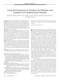


© Copyright 2026