
Toward a Theory of Non-linear Transitions from Foraging to Farming
Center for Behavior, Institutions and the Environment
CBIE Working Paper Series
#CBIE-2015-004
Toward a Theory of Non-linear Transitions from Foraging to Farming
Jacob Freeman
Utah State University
Matthew Peeples
Arizona State University
John M. Anderies
Arizona State University
April 7, 2015
The Center for Behavior, Institutions and the Environment resides in the School of Human Evolution and Social Change
at Arizona State University. CBIE can be found on the internet at: http://csid.asu.edu. CBIE can be reached via email
at [email protected].
c
2015
J. Freeman. All rights reserved.
Toward a Theory of Non-linear Transitions from Foraging to Farming
Jacob Freemana , Matthew Peeplesb , John M. Anderiesc ,
a The
Department of Sociology, Social Work and Anthropology, Utah State University;
of Human Evolution and Social Change, Arizona State University, Tempe, AZ 85287-2402, USA;
c Center for Behavior, Institutions and the Environment, School of Human Evolution and Social Change,
Arizona State University;
b School
Corresponding author:
Jacob Freeman
The Department of Sociology, Social Work and Anthropology
Utah State University
[email protected]
Abstract:
The evolution of agricultural economies requires two processes: 1) the domestication of plants and 2)
specialization in domesticates at the expense of hunting and gathering. Yet, in the literature,
domestication receives the lions share of attention while theories of specialization in domesticates lag
behind. In this paper, we integrate ideas from human behavioral ecology with tools from dynamical
systems theory to study the effects of ecological inheritance on the transition from foraging to farming.
Ecological inheritance is an outcome of niche construction and our study provides a formal link
between foraging theory and niche construction. Our analysis of a dynamic model of foraging and
farming illustrates that strategies for the optimal allocation of effort to foraging and farming can lead
to the emergence of multiple stable states. The consequence of this is that low-level farming optimizes
subsistence (e.g., minimizing the effort required to meet a subsistence goal) in a forager-resource
system over a few years, but makes the whole system vulnerable to punctuated change over decades
due to rare events. We use the insights of our model to propose a general ecological framework to
explain the evolution and diversity of transitions from foraging to farming.
Keywords:
Agricultural change, Niche construction, Human behavioral ecology, Foraging theory, Resilience
Toward a Theory of Non-linear Transitions from
Foraging to Farming
Jacob Freeman∗
Matthew Peeples †
John M. Anderies ‡
Abstract
The evolution of agricultural economies requires two processes: 1) the domestication of plants
and 2) specialization in domesticates at the expense of hunting and gathering. Yet, in the literature, domestication receives the lion’s share of attention while theories of specialization in
domesticates lag behind. In this paper, we integrate ideas from human behavioral ecology with
tools from dynamical systems theory to study the effects of ecological inheritance on the transition from foraging to farming. Ecological inheritance is an outcome of niche construction
and our study provides a formal link between foraging theory and niche construction. Our
analysis of a dynamic model of foraging and farming illustrates that strategies for the optimal
allocation of effort to foraging and farming can lead to the emergence of multiple stable states.
The consequence of this is that low-level farming optimizes subsistence (e.g., minimizing the
effort required to meet a subsistence goal) in a forager-resource system over a few years, but
makes the whole system vulnerable to punctuated change over decades due to rare events. We
use the insights of our model to propose a general ecological framework to explain the evolution and diversity of transitions from foraging to farming.
Keywords: Agricultural change— Niche construction— Human behavioral ecology—
Foraging theory— Resilience
1
2
3
4
5
6
7
8
9
10
11
12
Niche construction and its legacy–ecological inheritance–are integral to explain the adoption
of domesticated plants by hunter-gatherers [1–9]. This is intuitive. The adoption of domesticated
plants is one of the most studied problems in anthropology, particularly as an outcome of humanenvironment interactions (e.g., 4, 7, 10–28). The long standing justification for this intensity of
research is that the adoption of domesticated plants underlies major changes in the evolution of
human societies, such as the emergence of inequality and sociopolitical hierarchies (e.g., 29; 17;
21, p. 3; 25, p. 3; 26, p. 1). However, the evolution of political hierarchy and inequality are not correlated with the adoption of domesticated plants per se, but are often coincident with specialization
in the production of domesticated plants at the expense of hunting and gathering [17, 24, 30–33].
Thus, a fundamental question is why, once domesticated plants became part of the subsistence
base, did some people increase their time invested in farming at the expense of hunting and gathering while others engaged in a persistent mix of foraging and low-level farming [24, 32, 34–39]?
∗ The
Department of Sociology, Social Work and Anthropology, Utah State University
School of Human Evolution and Social Change, Arizona State University.
‡ The School of Human Evolution and Social Change and School of Sustainability. Arizona State University.
† The
1
13
14
15
16
17
18
19
20
21
22
23
24
25
26
27
28
29
30
31
32
33
34
35
36
37
38
39
40
41
42
43
44
45
46
In this paper, we integrate ideas from human behavioral ecology (HBE) and dynamical systems
theory to study why individuals specialize in the production of domesticated plants at the expense
of hunting and gathering. Our integration of ideas from HBE and dynamical systems theory allows
us to investigate the effects of ecological inheritance. Ecological inheritance is a process whereby
the behavior of individuals today modifies an ecosystem; and, in turn, the fitness of individuals’
behaviors in the future is effected by the modified ecosystem that they ‘receive’ from their ancestors
[40, p. 13]. Ecological inheritance is product of niche construction, which is simply the ability of
organisms to “shape environments to states that are suited to their biology (and less frequently to
states that are not)” [41, p. 221].
Our work contributes to understanding the coevolution of subsistence strategies and ecosystems. Specifically, we use the insight gained from a dynamic model of optimal foraging and farming to develop expectations for how ecological inheritance may result in different evolutionary
trajectories of food production strategies. We argue that HBE provides an overarching framework
to understand specialization in domesticates at the expense of hunting and gathering. However, the
feedback dynamics caused by niche construction can generate non-intuitive trajectories of evolution, and dynamical systems models are a critical tool for extending models drawn from optimal
foraging theory to understand such possibilities.
Foraging models, Ecological Inheritance, and Non-linear Trajectories
In HBE, many explanations for changes in human behavior are grounded by optimal foraging
models (OFM) (42, 43; see also 44). Such models are a useful starting point, but are not sufficient
to explain specialization in domesticates at the expense of hunting and gathering. To see why,
please consider the following example.
Barlow [34] proposes an OFM to describe investment in the production of domesticates at the
expense of hunting and gathering. With just a few assumptions, this model provides a partial explanation for when foragers will choose to invest in farming at the expense of foraging. Most relevant
here: 1) Individuals can invest their time in two mutually exclusive food producing activities, cultivating maize (the dominant domesticated plant in prehistoric North America) and foraging for wild
foods. 2) individuals only have so much time that they can use to produce food, thus ls + lc ≤ l.
Where l is the maximum amount of effort (in units of time) that an individual can devote to producing food, and ls and lc are the effort spent foraging and cultivating, respectively. (3) Individuals
attempt to maximize their rate of energy gain because this maximizes their fitness.
Given these assumptions, we can rewrite Barlow’s [2006] model in a compact form. Individuals
obtain an output of energy described by the following equation:
A(ls , lc ) = As (ls ) + Ac (lc )
47
48
49
50
51
(1)
where A(ls , lc ) is the total energy gained from foraging and farming; As (ls ) is a function that describes the energy gained from foraging; and Ac (lc ) is a function that describes the energy gained
from cultivating. When individuals maximize output subject to the time allocation constraint
above, it is assumed that they fully utilize their labor. Thus, the “≤” in the labor constraint becomes equality which leads to ls + lc = l or ls = l − lc . Hence, we can eliminate ls from equation
2
52
53
54
55
56
57
58
59
60
61
62
63
64
65
66
67
68
69
70
71
72
73
74
75
76
77
78
79
80
81
82
83
84
85
86
87
88
(1) an rewrite equation (1) as
A(lc ) = As (l − lc ) + Ac (lc ).
(2)
A0 (lc ) = −A0s + A0c = 0
(3)
A0s < A0c .
(4)
Differentiating output with respect to lc yields the first order conditions for a maximum, i.e.
which leads to a well-known condition in economics: at the optimal labor allocation, the marginal
productivity of labor in different occupations is equal, (i.e. A0s = A0c ). From this basic result comes
Barlow’s [2006] decision rule for when to cultivate maize:
This rule stipulates that individuals allocate effort to the cultivation of maize once the marginal gain
from the next unit of effort so spent is greater than the opportunity cost of that unit of effort spent
foraging [34, p. 96]. Thus, a decline in the marginal returns from foraging should spur investment
in cultivating maize and vice versa.
While a productive start, the model above needs further development. The most relevant reason
to our discussion is as follows. The model does not explicitly describe why the marginal returns
from either foraging or farming may increase or decrease. The causes of such changes could be
either endogenous or exogenous processes that change much more slowly than decisions about
how much time to invest in foraging and farming. For instance, on the foraging side of the equation, we can imagine that climate change may drive the productivity of important wild resources
down, leading to the adoption of more agriculture (if the climate change did not similarly affect the
marginal productivity of cultivating maize). Alternatively, population growth could lead to the depletion of wild resources, which would decrease the marginal rate of return from foraging relative
to farming; this possibility invokes ecological inheritance as a causal mechanism [3, p. 315].
A qualitative appeal to ecological inheritance as a causal mechanism glosses over the possibility that ecological inheritance results in non-linear trajectories of change in many systems [40,
p. 20-21]. Equation (4) assumes that foraging and farming are mutually exclusive, both as activities and in their effects on ecosystems. For an individual who makes decisions over a time scale of
months, this might be reasonable. However, over decades, the foraging and farming decisions of
many individuals likely creates interactions and interdependencies between foraging, farming and
ecosystems. For example, clearing land to plant crops over decades might positively or negatively
effect the productivity of wild resources; in turn, this interaction effect would determine how individuals should best allocate their effort to foraging or farming. The interdependency of foraging
and farming decisions with the productivity of an ecosystem could result in strong non-linearities
and threshold effects in the dynamics of human-environment interactions.
There are several potential reasons that the evolution of food production strategies may exhibit
such dynamics. However, our concern here is the potential effect of a specific type of non-linear
feature in social-ecological systems–the emergence of multiple stable states and thresholds–on the
evolution of subsistence strategies (e.g., 15, 45–49). Multiple stable states refers to the idea that
there are discrete ways that an ecological or social-ecological systems could be organized under the
same environmental conditions (e.g. hunting and gathering or agriculture) [50–54]. The emergence
of multiple stable states is important because their presence in a system could lead to transitions
3
89
90
91
92
93
94
95
96
97
98
99
100
101
102
103
104
105
106
107
108
109
110
111
112
113
114
115
116
117
118
119
120
121
122
123
124
125
126
127
128
129
130
from foraging to farming that are punctuated, difficult to anticipate, and very costly to reverse.
Thus, the emergence of multiple stable states under some regimes of ecological inheritance and
not under others is likely a factor that determines why systems of low-level food production follow
different evolutionary trajectories (e.g., smooth and continuous versus punctuated).
Multiple stable states
Figure 1 is a heuristic for understanding how systems with multiple stable states differ from those
with a single state or equilibrium. An equilibrium for a dynamical system is the “state” to which the
system tends over long time periods (e.g., a pendulum, after given an initial push will eventually
end up still, and hanging down). The value of this state can change as parameters that define
the system change (e.g., the length of the pendulum or the gravitational constant). The curves in
figures a-c show how the equilibrium of a system may change as an ecological parameter changes,
and the blue dots represent the equilibrium solution for a dynamical system for a given value of
the ecological parameter (e.g. solar flux, soil fertility, temperature, etc.).
In systems with a single possible equilibrium, there is a continuum of states that the system
can occupy (Figure 1a and 1b). The consequence is that evolutionary change is continuous and
reversible. Alternatively, in a system with multiple stable states (Figure 1c), there are multiple
equillibria that a system may occupy (i.e., multiple potential solutions to a system of equations
for a given set of parameters, two blue dots for the same parameter value). The consequence
is that evolutionary change is sometimes continuous and reversible, but may also be punctuated,
difficult to reverse, and difficult to anticipate. To illustrate these differences between systems,
please consider the following two examples.
First, assume that the choice an individual has to make in Barlow’s [2006] model is whether to
allocate time to cultivating maize or harvesting mesquite beans (a seed that falls from a mesquite
tree). Abstracting away from the issue of processing time for the moment, the marginal rate of energy gained from mesquite is determined by the density of mesquite trees. This is because the density of trees determines how long people must search for beans. By analogy, the density of mesquite
trees is the ecological parameter in Figure 1a or b (the x-axis) and time devoted to mesquite collection is the state variable (y-axis). This implicitly assumes that the density of mesquite changes
much more slowly (e.g., years) than decisions about the effort to invest in collecting beans (e.g.,
days-to-months). The black curves, again by analogy, represent the equilibrium time invested in
collecting mesquite at each given density of mesquite trees. As the density of mesquite declines,
selection pressures should favor decreasing labor, at equilibrium, in the collection of mesquite (the
blue dot moves down an to the right in 1a or 1b). Given the assumption of the model, a decline
in effort devoted to mesquite at equilibrium necessarily implies an increase in the production of
maize. In sum, there is a continuum of unique labor allocations to the collection of mesquite determined by the density of mesquite; the change in investment is continuous and reversible, and,
thus, labor allocation to farming also changes along a continuum.
Second, let’s continue the mesquite and maize theme to provide a concrete illustration of the
dynamics summarized in Figure 1c. Flannery [15] proposes that there are tradeoffs between clearing mesquite forests to plant maize and collecting mesquite beans. Flannery [15, p. 505] states,
“With maize crossing the the 250 kg/ha threshold, a new loop in the system was established; mesquite trees were cut down to make way for maize, and although preceramic
4
(a)
System state
k
{
Ecological parameter
(b)
System state
k
{
Ecological parameter
System state
(c)
k
{
k
{
250 kg/ha
Ecological parameter
Figure 1: Figures designed after Scheffer [53]. The black curves represent all of the possible equilibrium
states of a system for a given ecological parameter. The blue dots represent a unique equilibrium solution.
The arrows indicate the direction that the system will move over time if it is not in equilibrium.
5
131
132
133
134
135
136
137
138
139
140
141
142
143
144
145
146
147
148
149
150
151
152
153
154
155
156
157
158
159
160
161
162
163
164
165
166
167
168
169
170
171
172
peoples continued to collect mesquite pods, they were harvesting from ever dwindling
Prosopis groves. Instead of propagating mesquite seeds by their collecting and threshing behavior, they were propagating maize kernels by eliminating mature mesquite.”
In this example, the ecological parameter is the productivity of maize controlled by the selective
breeding practices of early Mesoamerican forager-farmers. The equilibrium state is the amount of
area covered by mesquite, which determines the abundance of mesquite beans.
Now we can analogize Flannery’s proposition to Figure 1c. An increase in the average productivity of maize (x-axis) causes a decrease in the level of effort devoted to the collection of
mesquite at equilibrium (the blue dot moves down and to the right). This occurs because individuals choose to plant more maize and cut down mesquite as the productivity of maize increases. In
this case, the 250 kg/ha threshold is marked by the thick red line. Once maize productivity hits
this threshold, farmers rapidly shift toward a low effort invested in collecting mesquite at equilibrium (all of the points on the lower right thick curve to the right of the shaded area. In Flannery’s
proposition, the reason the shift between equillibria occurs is because, once maize productiviy hits
250 kg/ha, deforestation and seed consumption decrease the rate of mesquite reproduction past a
critical threshold. The implication is that farmers move from a low level of effort to a high level
of effort devoted to the production of maize, and skip over intermediate levels of investment (the
dashed curve). In this case, the shift from low-level farming to intensive farming is punctuated and
costly to reverse. However there is more to the story.
Figure 1c helps illustrate that Flannery’s proposition is missing a crucial element. When the
ecological parameter (here the productivity of maize) falls within the shaded zone, the system is
vulnerable to a variance induced transition. This is because deforestation and consumption decisions are not solely controlled by the productivity of maize (the ecological parameter). There are
shocks that constantly perturb an ecological system generated by dynamics such as El Nino-La
Nina weather cycles and pest cycles. For example, a disease outbreak could shock a mesquite forest and cause a decline in mesquite forest cover. In the shaded area of Figure 1c, this shock would
stimulate individuals to compensate by growing more maize despite the fact that productivity is,
on average, below the 250 threshold. This behavior, in turn, would drive the rate of mesquite reproduction too low for the forest to recover. Forager-farmers would then end up in an environment
with a low density of mesquite trees, and their high investment in the production of maize would
keep the forest from recovering. In this situation, the transition is not only punctuated and difficult
to reverse, but also difficult to anticipate based on forager-farmers’ prior knowledge of the system.
The coupled processes of niche construction and ecological inheritance can lead to multiple
stable states and critical thresholds. The consequence of multiple stable states is that two mechanisms may generate a punctuated shift from to foraging to farming: 1) crossing a parameter
threshold (e.g., the 250 kg/ha line) through a slow process internal to a subsistence system, like
seed selection, or 2) crossing a state variable threshold (the dashed black curve) via a fast external
shock like a La Ni˜na episode. This second mechanism is captured in the example above when
forager-farmers, combined with a pest outbreak, deplete the density of mesquite just enough (past
the dashed curve in the shaded area) that they cause a regime shift. In short, the emergence of multiple stable states–due to niche construction and ecological inheritance–may effect the trajectory
of evolution that a system follows.
6
173
174
175
176
177
178
179
180
181
182
183
184
185
186
187
188
189
190
191
192
193
194
195
196
197
198
199
200
201
202
203
204
205
206
207
208
209
210
211
212
Questions
Two questions follow from our discussion: 1) Under what ecological and social conditions might
the optimal allocation of effort to foraging and food production cause multiple stable states to
emerge? And, if multiple stable states emerge, 2) what variables could create different trajectories that the evolution of food production follows? To contribute to answering these questions
we develop and analyze a dynamic model in the spirit of Barlow’s OFM and Flannery’s insights
regarding the interdependency of humans and ecosystems. Our questions hone in on the consequences of niche construction and ecological inheritance for the evolution of food production at
the expense of hunting and gathering.
A Dynamic Model of Time Allocation to Foraging and Farming
Our goal is to construct a model with the simplest possible assumptions to capture the biological
realism of niche construction and ecological inheritance. In particular, we want to capture, in a
minimal way, the interdependencies of foraging, farming, and the productivity of an ecosystem.
As we note in section six below, our stylized model has the analytical power to explore alternative
scenarios of niche construction and ecological inheritance. A more complex model would make
this more difficult because complexity necessitates a sacrifice of analytical power. For our argument here, analytical power is more important than model complexity, and, thus, we have chosen
to keep the model as simple as possible.
Our stylized model has two components: forest reproduction and growth and time allocation
to foraging or farming. We couple these two components to develop a dynamic model of time
allocation to foraging and farming in a forest ecosystem under three basic assumptions.
1. The individuals in our model are households. The household is a basal cooperative economic
unit in many forager-farmer and forager societies. In particular, a male and female pair or
pairs form the core of a group who performs complimentary subsistence activities. For
example, Holmberg [1950, p. 124] states “the nuclear family...is the fundamental economic
unit among the Siriono.” He goes on: “Hunting is largely a family affair, as are fishing
collecting and agriculture” [55, p. 124]. These types of observations are common from
diverse places such as the American Southwest, as among the Yavapai [56] to the the islands
of Indonesia, as among the Nuaulu [57].
2. We assume that households may choose to produce two staple resources: seeds produced by
trees (e.g., nuts like acorns or the mesquite beans mentioned above) and/or a domesticated
plant, which, for concreteness we call maize. It is common in the ethnographic record for
seeds or hearts produced from trees to provide a staple of forager and forager-farmer diets.
Examples include Pi˜nyon pine nuts in the Great Basin of North American [58], palm hearts
in South America and the Pacific (e.g., 55, 57, 59), and acorns in California [60]. The keys
here are 1) decisions are interdependent because clearing trees for agriculture effects the
production of seeds, and 2) there is a decision to make: How much effort is best allocated to
the production of each?
3. Territory is open access. Open access means that there are no rules that limit who, when, and
where trees may be cleared to plant and who, when, and where seeds may be collected. Our
7
213
214
215
216
217
218
219
220
implicit rules are simply ‘you harvest, you own’ and ‘you clear, you own.’ This means that
once a resource is harvested, or a plot of land is cleared, the resource is used by the household
that did the harvesting or clearing. For example, among Shoshoni foragers in the Great Basin
of North America, Steward [1938, p. 253] tells us that “once work had been done upon the
products of natural resources they became the property of the person or family doing the
work.” Again, among the Siriono Holmberg [55, p. 44] states that property is “limited to the
immediate possession, by a family, of a garden plot, by virtue of having cleared and planted
it.”
State Variables
s(t)
p(t)
Parameters
rj
Kp
ds
N
dc
c
K
hi
Ai
β
li
l
Interpretations
The density of seeds (biomass/area) at time t
The density of trees (biomass/area) at time t
Interpretations
The rate of resource regeneration where j ∈ {p, s}
Carrying capacity of trees
natural seed depletion rate
Density of households
Rate of tree clearance
Land cleared of trees (under cultivation)
Minimum daily energy return rate
Per capita harvest of resource i in s,c
The productivity of labor in resource i in s, c
Decay in returns to labor due to search time
Labor directed toward resource i in s, c
Total available per capita labor
Table 1: Model state variables and parameters
221
Forest reproduction and growth
222
We define the density of seeds and trees at time t with a set of ordinary differential equations:
s˙ = rs p − ds s
p˙ = r p s(1 − p/K p ).
223
224
225
226
227
228
229
(5)
(6)
This set of equations captures a minimal set of processes to generate a biologically defensible
story about the reproduction and growth of trees. The change in seed biomass (s)
˙ is the intrinsic
production of seeds (rs ) multiplied the density of trees in a forest (p) less the rate of seeds depleted
by animals and decay (ds s). In turn, the change in tree biomass per unit area ( p)
˙ is the logistic
growth function. The intrinsic growth of trees increases in proportion to the density of seeds in the
forest (r p s), and the growth limiting effects of intraspecific competition (K p ) constrains the growth
of trees. Here K p sets the area that households can use at time t. This means that when we speak
8
230
231
232
233
234
235
236
237
238
239
240
241
242
243
244
245
246
247
248
249
250
251
252
253
254
255
256
257
258
259
260
261
262
263
264
265
of the number of households at time t (N(t)), we are referring to a density. N(t) is best thought of
as the ecological footprint of households, given their technology; when N(t) = 0, humans have no
footprint in the forest.
Harvest and time allocation
Now that we have defined the ecosystem, we posit a set of rules that define an evolutionarily
sensible strategy for how households allocate their effort to the production of seeds or maize. To
determine the best allocation of effort to foraging and farming, we must first define the harvest of
seeds and maize.
We make three additional assumptions to define the per capita harvest of households. First, seed
output displays diminishing returns. Diminishing returns occur because the more seeds that one
gathers, the farther one must travel to gather more seeds (e.g., 61, 21-33; 62). Thus, as seeds are
depleted, an ever higher proportion of time is devoted to searching, which decreases the marginal
productivity of effort. Second, we assume that agricultural technology exhibits constant returns to
scale and that large scale cooperation is not necessary (like maintaining large irrigation ditches) to
produce maize. All else equal, this means that one extra day of labor invested in the cultivation of
maize results in a one unit increase in yield. The consequence of this assumption is that decisions
about how much time to invest in cultivation at the level of each individual household adds up
reasonably well to the aggregate level of cultivation by all household. Finally, we assume that
households minimize their time devoted to the production of sufficient food to meet their demands
(which is equivalent to maximizing the rate at which they gain energy).
Given these assumptions, we define hc (t) and hs (t) as the per capita harvest from cultivation
β
and seed gathering, where: hs (t) = As (s)ls and hc (t) = Ac (p)lc . In these equations ls and lc are the
time devoted to gathering seeds and cultivating maize. As and Ac are functions that represent the
productivity of effort spent foraging and farming, and 0 < β < 1 captures the decreasing marginal
productivity of seed gathering. We assume that As (s) = s because, for a given level of effort, lower
seed density implies a lower number of seeds gathered, and Ac (p) = p, which implies that soil
fertility scales linearly with tree density. This soil fertility assumption follows from the idea that
lower tree density is associated with shorter fallow periods and, thus, shorter times for trees to
regenerate soil nutrients. The effect of these last two assumptions is that we can replace As (s) and
β
Ac (p) with s and p, respectively. Thus, hs (t) = sls and hc (t) = plc . The per capita harvest of seeds
and maize depends on the abundance of seeds (s) and trees (p) (which we defined in equations (5)
β
& (6)) multiplied how much effort that a household invests in foraging (ls ) or farming (lc ), respectively. These simple harvest functions allow us to capture, in a minimal way, the interdependency
of foraging and farming–or at least the harvest of seeds and cultivation of maize.
We determine how much effort should be allocated to foraging and farming by solving a constrained optimization problem:
minimize lc + ls
subject to: lc + ls ≤ l
β
Ac lc + As ls − K ≥ 0
9
(7)
(8)
(9)
266
267
268
269
270
271
272
273
274
275
where l is the total time available, and K is the minimum caloric goal per person per day to meet
biological, reproductive and social needs. The constrained optimization problem simply says:
given that you have l total units of labor available per time period, produce K for that time period
with as little of your time budget allocated to foraging and farming as possible.
Box 1 presents the solution to the constrained optimization problem households face. The solution defines a set of decision rules for allocating effort to foraging and farming. Our decision set
is a heuristic that tells a household, at each time step, to check the optimal allocation of effort and
then allocate effort optimally if doing so does not violate the effort or minimum calorie constraints
noted above. The heuristic allows a household to converge on the best mix of foraging (ls ) and
farming (lc ) that meets K in the shortest amount of time whenever possible.
276
277
[BOX 1 HERE]
278
280
281
282
283
284
285
286
287
288
For example, Figure 2 illustrates five potential cases or ways that a household might allocate
labor at any given time t, given the productivity of the ecosystem at that time. The value ls∗ is the
point at which the marginal productively from cultivating is greater than the marginal productivity
from gathering seeds. In case 1 a household can meet their energy constraint, K at a point that
is less than ls∗ ; thus, the household is a hunter-gatherer household. In case 2, it is optimal for a
household to gatherer seeds until ls∗ and then cultivate maize until their energy constraint is met,
K. Thus, the household is a low-level food producer. In the model, a household could move
continuously between cases until they converge to some kind of an attractor. The main point is that
the optimal allocation of labor changes over time as the productivity of the ecosystem changes. We
define the interdependency of foraging, farming, and the ecosystem below.
K
1
Total Output
279
4
2
3
5
ls∗
Total Labor
l
l
Total Labor
ls∗
Figure 2: Graphic depction of the optimization problem faced by households. When the marginal benefit
of cultivation (slope of blue line) exceeds the marginal benefit of gathering seeds (slope of tangent to red
curve) swith to cultivtaion. This occurs at ls∗ , equation (16), Box 1. 1: Highly productive wild resource,
never cultivate, set ls = ls , subsistence constraint K easility met. 2: Set ls = ls∗ and lc = lc . It pays to
cultivate, and the subsistence constraint K is met. 3: Set ls = ls∗ and lc = l − ls∗ . It pays to cultivate, but the
subsistence constraint K is not met. Cases 4 and 5: It never pays to cultivate because l < ls∗ . The subsistence
constraint K may (case 4) or may not be met (case 5) depending on the productivity of the resource.
10
289
290
291
292
293
294
295
296
297
298
299
300
301
302
303
304
305
Coupling the ecosystem with harvest and time allocation
The production of food creates two niche constructing activities in our model (i.e., feedbacks between time allocation and the ecosystem): gathering seeds hs (t) and the harvest of maize hc (t).
The effect of gathering seeds on the dynamics of the forest is obvious, the more seeds that individuals gather, the lower the reproductive rate of trees in the forest. The total harvest of seeds in the
model is Nhs (t); the number of households multiplied by each household’s harvest of seeds. Similarly, given our production function of hc (t) = plc , to cultivate maize a household must choose
how many trees to clear, which effects the reproductive rate of the forest, as well as the fertility of
soil. Thus, households make a clearing decision: If the amount of cleared land is insufficient for
the desired production of maize, then land must be cleared. We define c(t) as a household’s rate of
land clearing at time t. Total tree clearing, Nc(t) is the number of households multiplied by each
household’s rate of clearing. Finally, we assume that land is cleared at a rate proportional to the difference between the desired cleared area and the available cleared area: c(t) = dc (Acd /Aca ). Where
dc is a measure of how effectively a household clears trees per unit effort and how responsive they
are to deviations of Acd /Aca , the ratio of area that needs cleared to the area already cleared, away
from K p .
We can now couple the behavior of households with the growth and reproduction of the forest:
s˙ = rs p − ds s − Nhs
p˙ = r p s(1 − p/K p ) − Nc.
306
307
308
309
310
311
312
313
314
315
316
317
318
319
320
321
322
323
Given seed and tree densities, s(t) and p(t), at time t households make a decision about how much
effort to allocate to foraging (ls ) and farming (lc ), which determines hs (t) and c(t). In turn, hs (t)
and c(t) affect the future values of s(t) and p(t) through equations (10) and (11) and, thus, the
best allocation of effort to foraging and farming in the future. In sum, the fitness of a household’s
decisions now depends, in part, on the forest that it “inherits.”
The Evolution and Resilience of Low-level Food Production
Our analysis indicates that 1) as our model households attempt to behave optimally, their niche
construction and its legacy, ecological inheritance, generate multiple stable states: a productive
state and an impoverished state. Once multiple stable states emerge, households face the risk that
they may get pushed into the impoverished state. This risk is a feature of the ecosystem inherited
from previous generations. 2) As households cultivate more maize, the resilience of the productive
state decreases, and the risk of the system flipping into the impoverished state increases. Thus, in
the short-run (a few years), it is optimal to allocate effort to the cultivation of maize as a strategy
to mitigate diminishing returns from foraging; however, in the longer-run (decades), the system is
more vulnerable to a punctuated state change that is difficult to anticipate. 3) It is less costly for
households to reverse between foraging and farming when cultivation is 1-40% of the diet. However, once the 40% threshold is approached and crossed, it is likely difficult to go back to low-level
food production.
324
325
(10)
(11)
[BOX 2 HERE]
11
326
327
328
329
330
331
332
333
334
335
336
337
338
339
340
341
342
343
344
345
346
347
348
349
350
351
352
353
354
355
356
357
358
359
360
361
362
363
364
365
366
367
368
369
The emergence of multiple stable states
Figure 3 is a set of phase plane plots that illustrates the inter-relationships between seed and tree
density over time for three different values of population (N): N = 0, N = 1.1, and N = 1.85. The
green and orange curves on each of the graphs are the isoclines. The isoclines are all of the points
at which seed density or tree density are not changing (i.e., s˙ = 0 or p˙ = 0). Where these curves
intersect, the system is in equilibrium because s˙ = 0 and p˙ = 0. An equlibrium may be stable,
also known as an attractor, or unstable, also known as a repellor. An attractor is a collection of
equilibria to which a system is likely to return over the long-term if perturbed. A repellor is a
collection of equillibria that a system is likely to move away from over the long-term, if perturbed.
Figure 3a has one attractor where the isoclines intersect (s = 1, p = 1) and, thus, one stable
state. The stable state is “pristine” because, at N = 0, humans do not have an ecological footprint
in the system. The stable state is globally resilient. Resilience refers to how much environmental
change a system can absorb and still maintain its feedback structure [63]. For example, the black
arrowed curves on Figure 3 illustrate how a system evolves over time for a given set of initial
conditions. To illustrate, please follow the curve labeled “I” on Figure 3a. This system starts at a
seed density of s = 0.25, and a tree density of p = 0.3. Over time, the trees produce seeds, which
sprout and grow into trees and the forest recovers toward the pristine state (s = 1, p = 1). In the
long-run, the stable state in this environment is globally resilient because no matter where we start
the system, it will always move toward s = 1, p = 1 over the long run.
Please hold-on to the idea that resilience is a long run characteristic of an attractor. In real
systems, perturbations constantly occur, for example, a pest outbreak in a forest that drives tree
and seed biomass down.
The black arrowed curves on Figure 3 help us imagine the consequences of perturbations. In
the case of the curve labeled “I”, we can imagine that a pest outbreak killed-off a bunch of trees in
one year, thus setting the initial conditions for the next year at s = 0.25, p = 0.3. In the short-run,
the pest outbreak depresses the biomass of the forest, but, at longer time scales (over a decade),
the forest moves toward the pristine attractor. In a real system, biomass may never actually get
to the pristine state because perturbations are constant. However, the system is globally resilient
because, over time, it continues to move back toward our “pristine” stable state. Thus, the black
arrowed curves help us understand the sets of initial conditions for which the forest will tend to
evolve toward a particular stable state.
In Figure 3b, we add some humans to the ecological system (N = 1.1). Now, the collection of
seeds and, potentially, the clearance of forest by households can affect the long-run biomass of the
ecosystem. There are two consequences.
First, the pristine stable state is no longer pristine; the attractor moves down and to the left. At
this ‘productive’ attractor, it is optimal for households to expend 12 % of their total available effort
(i.e., 12 % of their subsistence time-budget) to gather seeds; and this allocation of effort allows
households to achieve their daily caloric goal (K) in a minimum amount of time. In the productive
state, households do not work very long and can invest a lot of time in other activities that enhance
fitness.
Second, when N = 1.1, the system displays multiple stable states, and the harvest behavior of
households (collecting seeds) introduces the subtle risk that a perturbation may drive the system
into an ‘impoverished’ attractor. The impoverished attractor on Figure 3b is separated from the
productive attractor by a repellor (the blue square). In this multiple stable state environment, now
12
(a)
Seed density (s)
1
(d)
0.8
0.6
0.4
I
0.2
0
0
0.2
0.4
0.6
0.8
1
Tree density (p)
(b)
Seed density(s)
1
(e)
0.8
0.6
0.4
I2
0.2
0
0
0.2
0.4
0.6
0.8
1
Tree density(p)
(c)
Seed density (s)
1
(f)
0.8
0.6
0.4
0.2
0
0
0.2
0.4
0.6
0.8
1
Tree density (p)
Figure 3: Phase plots: All parameters are held constant at default values except population (N). a-N = 0;
b-N = 1.1; c-N = 1.85. The circles highlight stable attractors. The square in graph b highlights a repellor.
Each phase plot is paired with a stability landscape (a-d; b-e; c-f).
13
370
371
372
373
374
375
376
377
378
379
380
381
382
383
384
385
386
387
388
389
390
391
392
393
394
395
396
397
398
399
400
401
402
403
404
405
406
407
408
409
410
411
412
if a pest outbreak reduces tree and seed biomass to the point labeled I2 , the system will move
toward the impoverished attractor over the long-run. This occurs because as the biomass of the
forest goes down, it suddenly becomes optimal for households to invest in both clearing forest to
plant maize and collecting seeds (e.g., a shift from case 1 to case 2 in Figure 2). If the biomass of
the forest decreases too far (all sets of (s,p) left of the dashed blue line), a feedback loop between
seed gathering and clearing is initiated. Lower tree density leads to fewer seeds which means it
is optimal for households to clear more land to plant maize. The short term decision to clear land
leads to lower tree density which reduces seed density over the longer term. One can imagine how
this viscous feedback cycle could lead to the destruction of the forest.
However, at N = 1.1 the impoverished state is only impoverished in terms of the ability of
households to collect seeds. Each household can still obtain K; they simply are doing it by working
a lot harder than they would as pure foragers in the productive state. At the impoverished attractor,
households spend 71 % of their subsistence budget cultivating maize and 29 % gathering seeds.
In short, when N = 1.1, there are two stable states. In the productive state, households are
pure foragers who need not work very long. In the impoverished state, households are committed
farmers and work long hours. Note: if the system were hit by a large enough perturbation, we
would observe a regime shift from pure foraging at the productive attractor to fully committed
farming at the impoverished attractor! There is more to this story, however. The impoverished
attractor is not very resilient to further environmental change.
Figure 3c illustrates how sensitive the impoverished attractor is to increases in the ecological
footprint of households. In this setting, we have increased N to 1.85 and the system bifurcates.
The only attractor is the impoverished attractor, very near s = 0, p = 0. The destruction of the
forest occurs, in part, because of the feedback noted above where clearing decreases tree and seed
biomass, which makes cultivating a more optimal strategy so people clear more forest. The other
assumption that leads to the deconstruction of the forest is that soil fertility is proportional to
tree biomass. As the biomass of trees declines, the yield of maize per unit area declines. The
consequence: people need to clear ever more area to meet their desire for maize, but the fertility
of the soil is just too low to ever get enough food to meet K. Hence, once people flip to the
impoverished attractor, any small increase in population or decline in the productivity of trees (rs
& r p ) will cause large declines in the productivity of maize and decimate the productivity of the
ecosystem.
The long-run effect of low-level food production
The emergence of multiple stable states has a subtle but profound consequence. It is often optimal
for a household to engage in low-level food production at the productive attractor; however, when
households adopt low-level farming, the system looses resilience and becomes more vulnerable to
a flip from the productive to the impoverished state.
Figure 4 is a bifurcation diagram analogous to Figure 1c. This diagram is a tool for illustrating
how, holding other parameters equal, N affects the structure of the system. On the x-axis we have
plotted N, and on the y-axis we have plotted the percent of diet obtained from foraging (hs /K)
when the system is at equilibrium (i.e., s˙ = 0 and p˙ = 0). The thick black curves are all of the
productive and impoverished attractors that would emerge for given values of N. The dashed
curved is the collection of repellors that emerge for given values of N and separates the productive
and impoverished curves. The shaded area defines all of the values of N for which the system has
14
413
three equllibria (two attractors and a repellor).
1.00
productive harvest branch
6
Proportion of diet from seeds (hs /K)
0.75
0.50
6
The probability of a flip to the alternate attractor
(or regime shift) increases as the distance between
the stable productive branch and unstable branch decreases (double arrow lines)
?
?
unstable harvest branch
0.25
0.00
impoverished harvest branch
0.0
0.5
1.0
1.5
Population density, N (households/area)
2.0
Figure 4: Summary of the relationship between N and the proportion of the diet obtained from seeds at
equilibrium. The upper solid line represents all of the productive attractors; the dashed middle line, all
repellors (unstable branch), and the lower solid line all of the impoverished attractors. Shaded area defines
the parameter space in which a perturbation can cause the system to flip between attractors.
414
415
416
417
418
419
420
421
422
423
424
425
Figure 4 demonstrates that low-level food production is often optimal over the short term,
but also creates conditions that may lead to the rapid and difficult to reverse process of adopting
agriculture at the expense of hunting and gathering over the longer run. Reading from left-toright, as N increases, households in the productive state (the top left branch) remain pure foragers
until a threshold of about N = 1.25. At N = 1.25 households begin to cultivate maize as a minor
component of their diet, and the proportion of the diet from foraging begins to decline. Once
households begin to optimize by cultivating maize, small increases in N lead to fast decreases in
the proportion of the diet that comes from foraging (the productive harvest branch bends down
and to the right). However, foragers can only replace a maximum of about 40 % of their diet with
maize before the system bifurcates, and the only attractor is the impoverished state (i.e. the system
crosses a parameter threshold).
It is intuitive that households can replace declining returns from seeds with maize with little
15
426
427
428
429
430
431
432
433
434
435
436
437
438
439
440
441
442
443
444
445
446
447
448
449
450
451
452
453
454
455
456
457
458
459
460
461
462
463
464
465
466
467
disruption to their foraging system over the short run [34]. However, cultivating maize in response
to declining returns from foraging (caused here by increases in N relative to r p and rs ) means
that the system is more likely to flip over the long-run (i.e. cross a state variable threshold).
Given enough time, a big enough shock is sure to occur in most environments. To elaborate:
we can estimate the resilience of the productive attractor by estimating the size of the attractor.
We estimate size by calculating the Euclidean distance between the productive attractor and the
unstable harvest branch (the repellor) in Figure 4 [50]. As the size of the productive attractor
declines, the probability that a perturbation induces a regime shift increases. the point here is
that a one unit decline in the proportion of diet from foraging, at the productive attractor, induces
a decline in the size of the productive attractor that is greater than one. Thus, a perturbation of
similar size is more likely to induce a regime shift from the productive to impoverished attractor
as households supplement foraging with farming at the productive attractor.
In sum, the optimal allocation of effort to foraging and farming can make a system of low-level
food production vulnerable to a ‘flip’–caused, in part, by the very rules that allow individual’s
optimize their production of food. If the system flips into the impoverished state, the ecosystem
is vulnerable to degradation. The implication is that if a system flips, households either abandon
the area or engage in classic Boserupian responses. Boserupian responses are strategies that invest
labor in new niche construction activities and increase the productivity of land per unit area, as
well as decrease the need to further harvest trees (thereby improving soil fertility). Hence, at the
productive attractor, it is likely not very costly to increase or decrease effort in farming as perturbations (droughts, etc.) dictate year-to-year. However, if environmental variation initiates a flip
into the impoverished state, households have to leave or lock-in to a run away niche construction
strategy that mitigates declines in soil fertility. A central issue is whether households might ascertain from their knowledge of the environment that the risk of getting pushed into the impoverished
state is a novel feature of their social and ecological world. If so, they might be able to adapt to
longer-term variation and modify how they allocate effort in the short term; if not: look out!
So What?
Our work is motivated by a basic question. Why, once domesticated plants became part of the
subsistence base, did some people increase their time invested in farming at the expense of hunting
and gathering while others engaged in a persistent mix of foraging and low-level farming? One
way to answer this question is to use the tools of foraging theory and ask: When does an individual
maximize their fitness by investing in farming at the expense of foraging, and this has been a
productive line of research (e.g., 20, 64–67). However, the foraging models that anthropologists
typically use can benefit from further development (e.g., 27, 68). Foraging models, often, do
not account for the feedbacks caused by niche construction and, thus, the process of ecological
inheritance. Ecological inheritance is known to cause non-linear trajectories of evolution. An
important possibility is that ecological inheritance may result in multiple stable states, or ways that
humans could be organized to obtain food in a given environment. Multiple stable states can lead
to transitions that are punctuated, difficult to anticipate, and very costly to reverse.
Therefore, we have combined an optimization model with a dynamical systems model to study
the effects of niche construction and ecological inheritance. We asked two specific questions.
Under what ecological and social conditions might the optimal allocation of effort to foraging and
16
468
469
470
471
472
473
474
475
476
477
478
479
480
481
482
483
484
485
486
487
488
489
490
491
492
493
494
495
496
497
498
499
500
501
502
503
504
505
low-level food production cause multiple stable states to emerge, and if they do, what variables
should create different trajectories that the evolution of food production follows? The analysis of
our model provides an answer to the first question, and creates a more informed position to propose
an argument that may help answer the second question.
The model generates multiple stable states when the ecological footprint of households increases beyond a critical threshold (Figures 3b & 4). The emergence of multiple stable states has
four implications.
1. When a household behaves optimally in the short-run, this act exposes all of the households
to the risk of flipping from a productive state to an impoverished state over the longer run.
2. The risk of the system flipping emerges when households are still pure foragers, which opens
up the possibility that households may suddenly transition from full-time foraging to full
time farming. However, the full time farming at our impoverished attractor is very sensitive
to increases in population density or declines in the productivity of wild resources. Any
slight change will cause the system to move toward a completely denuded state.
3. The adoption of low-level food production in the productive state makes the whole system
more vulnerable to perturbations. The implication is that low-level food production is costly
to maintain (but see below).
4. The dynamics of our model provide a theoretical basis for defining low-level food production with domesticates as a space defined by a diet between 1 and 40% dependence upon
domesticates. Note: The 40% threshold is not a universal. The exact value would vary from
system to system, depending on the specifics of particular ecosystems. The key is the qualitative insight that there is a parameter threshold, and it will likely fall somewhere between
1 and 40% in many particular systems. Incidentally, there is empirical evidence that major
changes in the way households organize labor occurs cross-culturally at a threshold of about
35% dependence on domesticated plants [35].
The issue now is: Why do systems follow different trajectories of evolution on the path from
foraging to farming? To begin to use the insights from our model to answer this question, we
consider the transition from foraging to farming in the pi˜nyon-juniper forests of the Colorado
Plateau in the American Southwest. Our argument for this specific place then provides a point of
departure to speculate about why systems of food production may follow different evolutionary
trajectories.
An example to help consider the broader implications of the model
The Colorado Plateau is an arid region with elevations ranging between 1,500 and 3,000 meters.
The region is drained by the Colorado River and its tributaries, and is also dissected by numerous
small perennial and seasonal drainages. Many of these drainages form deeply incised canyons
bordered by high upland mesa tops. The upland mesa tops are, in most locations, dominated by
pi˜nyon and juniper trees. Over the course of prehistory, these highland mesa tops became the
primary settings occupied by prehistoric farmers across much of the Plateau.
17
506
507
508
509
510
511
512
513
514
515
516
517
518
519
520
521
522
523
524
525
526
527
528
529
530
531
532
533
534
535
536
537
538
539
540
541
542
543
544
545
546
The Colorado Plateau spans two archaeological cultures; the Ancestral Puebloan and the Fremont. Both Ancestral Puebloan and Fremont populations engaged in farming. One major distinction, however, is that while populations in the Ancestral Puebloan region were committed agriculturalists by about A.D. 700 or earlier in some places, populations in the Fremont region relied on
hunting and gathering, in many locations, throughout prehistory [64, 69]. Thus, while the transition to agricultural dependence appears to have been relatively complete in the Ancestral Puebloan
region, the occupation of the Fremont region represents more of a mosaic with different strategies
being used in different places over the long term. Our concern here is not with the initial arrival
of agriculture but the increased investment in agriculture and the development of new strategies,
including upland cultivation. The transition to upland cultivation occurred on several parts of the
Colorado Plateau, such as: the Mesa Verde/Northern San Juan region, Cedar Mesa, portions of the
Mogollon Rim, and areas along the Fremont and Green Rivers. This transition was variably timed
but primarily occurred between about A.D. 200 and A.D. 750 in the four corners (70, p. 128-129;
71) and as late as A.D. 1000 further north in portions of the Fremont region [72, 73].
Based on paleobotanical and settlement data, many researchers have suggested that the prehistoric agricultural systems in the pi˜nyon-juniper woodland mesa tops along the Colorado Plateau
involved a type of shifting cultivation. This method of cultivation involved the clearing of small
field areas, likely with fire, followed by planting in the cleared areas. This was followed by a long
fallow period when the woodland plots were allowed to regrow and soil nutrients regenerate (e.g.,
71, 74–81). Local transitions from foraging and other forms of agriculture to extensive cultivation
of upland mesa tops are interesting because explanations for this change are not straight forward.
Extensive shifting cultivation is less efficient than many other types of agriculture and foraging
[64, p. 80], it is risky [70, p. 135-136], and it is not locally sustainable [74–76]. So why did the
shift to extensive cultivation occur?
One way that we might answer this question is to directly analogize from the dynamics of
our model. Recall that we observed the possibility of a regime shift from pure foraging to farming, where over 70% of a household’s time budget was devoted to cultivation and the forest cover
severely declined (Figure 3b). In this argument, prehistoric foragers would have inadvertently
backed into the adoption of extensive cultivation. If this occurred on the prehistoric Colorado
Plateau, we would expect to see the punctuated adoption of extensive agriculture and a punctuated
denuding of pi˜nyon-juniper forests on mesa tops. Although, there does seem to be a punctuated
increase in commitment to extensive cultivation, particularly in upland contexts [71, 76, 82], declines in forest cover seem to have occurred much more slowly, as people became more committed
to agriculture. Further, in some locations, the the coordinated use of high frequency fires by households may have maintained a dynamically stable forest structure that was good for disturbance
loving plants such that are integral species in almost all agroecological systems in North America
(e.g., 83). This suggests that a more subtle argument is required to understand why people may
shift from low-level food production in which cultivation supplements foraging to a subsistence
system in which foraging compliments farming-where labor is organized first around the intensive management of small patches to insure against risk, even though foraging may still provide
substantial calories.
18
547
548
549
550
551
552
553
554
555
556
557
558
559
560
561
562
563
564
565
566
567
568
569
570
571
572
573
574
575
576
577
578
579
580
581
582
583
584
585
586
587
588
589
590
An argument
To build our argument, we combine the insights of our model with two empirical statements that
relate the structure of ecosystems to tradeoffs in the knowledge economies necessary to obtain a
reliable supply of food as a mobile forager versus a farmer.
First, Holling [84] provides empirical evidence that ecosystems are organized into a hierarchy
of structures (i.e. leaf, tree, patch of trees, habitat, landscape, biome) controlled by a handful of
processes that operate at distinct scales of space and time. The consequence is that animals face
a decision hierarchy [85]. Second, in part because of the hierarchical structure of ecosystems,
humans face a knowledge tradeoff. Farmers plant fields at the scale of a patch. The successful
production of crops depends on having a detailed knowledge of the soil conditions, flow of water,
and timing of temperature changes in the few patches where fields are planted. Mobile foragers,
alternatively, use landscapes. Thus, knowledge of different landscapes, each composed of multiple
habitats that are, in turn, composed of multiple patches is essential for human foragers to consistently produce food [86]. In short, farmers need a fine grained knowledge of patches, and foragers
need a coarse grained knowledge of landscapes to make decisions about where to locate in space
and time and invest effort to produce food.
The difference in the knowledge economies necessary to forage versus farm is significant. As
one uses more levels in the ecosystem hierarchy, the number of processes that affect the distribution
of resources increases. The consequence is that foragers need a generalizable system of knowledge
to encode information across many scales of space and time while farmers need a more partitioned
and textured knowledge of ecosystems. For example, Brown [87] documents that farmers living
in the same environment as hunter-gatherers partition their knowledge of plants and animals into
much finer categories. That is, for a forager, a flower is a flower, but for a farmer, a flower is a red
rose, yellow rose, daffodil, etcettera. The costs of obtaining information in the nested hierarchy
of ecosystem structures that humans exploit is very instructive for understanding this difference.
Foragers minimize the costs of collecting information across many levels of the ecosystem hierarchy by generalizing. In contrast, farmers minimize the risk of planting at the wrong time or in
the wrong location by investing in a fine grained knowledge of lower levels in the hierarchy, like
patches.
In our model, once foragers adopt low-level food production (less than 40% of the diet from
domesticates), the net effect of this behavior is to make the system vulnerable to a flip from the
productive to the impoverished state. In the context of the nested hierarchy of ecosystem structures
that human foragers encounter; we can extend this insight to make two related propositions. 1)
The effects of cultivating to supplement the diet obtained from foraging at the level of ecosystem
patches, scales-up to make habitats (much larger tracks of an ecosystem) vulnerable to a flip from
the productive to impoverished state. 2) The consequence of this is that while over a few of years
it appears optimal to supplement foraging with a little farming; this behavior makes it harder to
maintain a foraging system over decades based on coarse grained knowledge about a landscape.
The reason is this: now foragers must know how likely habitats are to flip into the impoverished
state in addition to everything else. Further, it may be very difficult to predict such flips. An easy
solution is to just farm more, but using the low-level strategy that we presumed in our model will
simply degrade natural capital and make a flip more likely. In this context, selection and copying
should favor a fine grained knowledge system that allows individuals to shift their subsistence
system to one committed to farming at or above the 40% line and minimizes the short to medium
19
591
592
593
594
595
596
597
598
599
600
601
602
603
604
605
606
607
608
609
610
611
612
613
614
615
616
617
618
619
620
621
622
623
624
625
term (years to decades) impact of farming practices on the degradation of the forest.
In the context of the Colorado Plateau, we might expect that once domesticates were introduced to mesa top forests, the shift to minimally committed agriculturalists may have been quite
rapid, stabilizing major tree depletion and more effectively allocating effort. However, once in this
committed agriculture regime was established, it may have locked-in and slowly evolved toward
ever more committed agriculture. In this regard the Fremont provides an interesting contrast. 1
Holding all else equal, it may be that the adoption of agriculture was most rapid in the areas with
the densest forests, and foraging remained dominant in other areas because of diverse ecosystem
types, including highly productive wetlands not characteristic of the Southwest US in general. In
the deserts of the Southwest US and Northern Mexico, only the eastern half of the Mexican state of
Chihuahua has somewhat analogous wetland formations, and maize was never adopted in this area
prehistorically. The bifurcation of a foraging and farming regime could have provided the adaptive
space for individuals to move between systems and give the impression of a stable low-level food
production system as described by our model (i.e., a system where household diet is between 1 40% dependent on agriculture) in the Fremont area.
Macroecology and Macroevolution
Our argument above provides a starting point from which to generalize. If low-level food production decreases the resilience of forager-resource systems, in general, across the hierarchy of
ecosystem organization: we propose that low-level food production is only weakly stable. Either
an increase in the costs of processing information will stimulate individuals to shift to a committed
agricultural way of life based on a knowledge system with a finer grained texture, or they will
abandon an area all together. The sum result is that low-level food production should be quite rare
in human societies.
Figure 5 demonstrates that low-level food production with domesticates is very rare in human
societies. Figure 5 is a histogram of the societies recorded in the Ethnographic Atlas [88] that
have subsistence information. There is a gap between hunting and gathering on the one hand and
farming on the other. Detailed study of this gap suggests that major changes occur in societies’ use
of resources at a threshold of about 30-35% dependence on farming. Farmers above this threshold
grow a high diversity of crops, seemingly set by the tolerance limits of crops in their environment;
however, farmers below this threshold only grow a few crops, usually a subset of crops grown
by their neighbors [89]. Further, above the threshold, farming societies tend to have one or more
formal weeding periods, and below this threshold no such formal institutions are observed [35,
p. 3011-3012]. These data do not test whether foraging regimes and committed farming regimes
are more resilient than low-level farming regimes, but they do something equally important. They
warrant the development of more rigorous study. Nonetheless, our model combined with our
1 The
idea that coordinated, high frequency burning maintains an open forest in a kind of dynamically stable state
[83] fits very well with the kind of transition that we argue occurs in knowledge economies-even though wild foods
still dominate the diet. The shift to a high management strategy and fine grained knowledge economy may increase the
resilience of a forest to shocks or at least keep resilience from going down any further. But the Upper Colorado system
discussed by Sullivan et al. [83] obviously was abandoned at some point. There may have been limits to how much
this strategy could effect the resilience of the forest across scales and, thus, reduce the uncertainty of food production.
Given a big enough shock (perhaps the Little Ice Age) many levels of the system might have experiences a flip and
contributed to abandonment.
20
626
627
knowledge argument indicates that low-level farming is a less resilient strategy than foraging and
committed farming.
0.20
Density of cases
0.15
0.10
the gap
0.05
0.00
0
20
45
70
Proportion of diet from agriculture
100
Figure 5: Histogram of the density of societies per binned level dependence on agriculture (domesticated
plants only).
628
629
630
631
632
633
634
635
636
637
638
639
640
641
642
643
644
645
Smith [2001] has warned us not to discount the groups in the “gap” in Figure 5, and he is correct. One reason that low-level food production regimes may develop and persist is that variation
in vegetation communities causes the effects of ecological inheritance on foraging economies to
diverge in space and time. For example, our model is a case in which niche construction causes a
particular directional effect on the productivity of wild resources and domesticates (controlled by
soil fertility). The directional effect is a double negative, harvesting seeds and clearing the forest
depletes the future productivity of trees and the soil. Ecological inheritance need not occur in this
manor. There are four possibilities: + +, + −, − +, and − −. We propose that holding other
factors equal, the trajectory of evolutionary change varies in predictable ways based on the directional effect of ecological inheritance in an ecosystem. That is, if two populations adopt low-level
farming, the trajectory of evolution for the population living in an environment with a double positive will be different from the trajectory of the population living in an environment with a double
negative. There are two ways to evaluate this proposition.
First, we could ask: what changes to the assumptions of the model developed above are necessary to generate large basins of attraction for low level farming? Using this strategy, the challenge
would be to build reasonable assumptions about the harvest behavior of forager-farmers that generate the four possible scenarios listed above. This strategy allows for the possibility of a more
precise description of what happens in each case (e.g., + + vs. + −) in terms of the trajectories
21
646
647
648
649
650
651
652
653
654
655
656
657
658
659
660
661
662
663
664
665
666
667
668
669
670
671
672
673
674
675
676
677
678
679
680
of change in different systems. For example, the systems might generate oscillations or chaotic
attractors, as opposed to stable equillibria, which may have physical meaning in some contexts.
Second, we could start with two empirical propositions 1) In the case of double positive effects,
the resilience of a low-level farming regime should be enhanced, and, thus, be more likely to
withstand perturbations. For example, the Nualulu of Indonesia might live in a double positive
setting. They plant and tend both wild and domesticated sego palms. The wild segos increase
in productivity in response to low-level clearing and burning conducted to cultivate domesticated
segos [57]. 2) In the case of a double negative, as in our model, the resilience of the low-level food
production regime should decline and we should see a bifurcation between ‘pure’ foraging and
minimally committed farming subsistence regimes. We could then take a representative sample of
the Ethnographic Atlas and classify each case according to the likelihood that low-level cultivation
will deplete vs. increase the key wild resources in an environment, and the effect of low-level
cultivation on soil fertility. This would be a coarse grained analysis, but it would allow us to divide
the sample into + +, + −, − +, and − −sets of cases. We would expect the frequency of low-level
food production to be highest in + + settings, second highest in + − and − + settings, and lowest
in − − settings.
Conclusion
It is trivial (almost tautological) to state that niche construction and ecological inheritance partly
determine the evolution of food production. Our goal in the work presented here is to understand
why the process of ecological inheritance, which is an outcome of niche construction, might cause
different evolutionary trajectories. We have read with great interest the recent debate over whether
human behavioral ecology provides an overarching framework for studying the adoption of domesticated plants (7–9, 90–92; see also 15 & 27 for an earlier version of the argument). We argue
that HBE provides an overarching framework to understand specialization in domesticates at the
expense of hunting and gathering. However, the feedback dynamics caused by niche construction
may cause non-intuitive trajectories of evolution, and dynamical systems models are a critical tool
for improving our understanding of such possibilities. In this paper, we have shown that multiple stable states occur when we include the process of ecological inheritance (caused by niche
construction) in a optimization model drawn from foraging theory/microeconomics. This model
illustrates that the optimality of individual foraging decisions over shorter time scales and the resilience of a system over longer time scales are both important for understanding the evolution of
food production.
Acknowledgments
We gratefully acknowledge the support of the NSF Dynamic Coupled Natural and Human Systems
Program (#CNH-1113991).
22
681
682
683
684
685
686
687
688
689
690
691
692
693
694
695
696
697
698
699
700
701
702
703
704
705
706
707
708
709
710
711
712
713
714
References
[1] Bleed, P. & Matsui, A. Why Didn’t Agriculture Develop in Japan? A Consideration of
Jomon Ecological Style, Niche Construction, and the Origins of Domestication. Journal of
Archaeological Method and Theory 17, 356–370 (2010).
[2] Crawford, G. W. Food Production and Niche Construction in Pre-Contact Southern Ontario
(2014).
[3] Laland, K. N. & O’Brien, M. J. Niche construction theory and archaeology. Journal of
Archaeological Method and Theory 17, 303–322 (2010).
[4] Rowley-Conwy, P. & Layton, R. Foraging and farming as niche construction: stable and
unstable adaptations. Philosophical Transactions of the Royal Society B: Biological Sciences
366, 849–862 (2011).
[5] Smith, B. D. Niche Construction and the Behavioral Context of Plant and Animal Domestication. Evolutionary Anthropology 16, 188–199 (2007).
[6] Smith, B. D. General patterns of niche construction and the management of ‘wild’plant and
animal resources by small-scale pre-industrial societies. Philosophical Transactions of the
Royal Society B: Biological Sciences 366, 836–848 (2011).
[7] Smith, B. A cultural niche construction theory of initial domestication. Biological Theory 6,
260–271 (2011).
[8] Smith, B. D. A Comparison of Niche Construction Theory and Diet Breadth Models as
Explanatory Frameworks for the Initial Domestication of Plants and Animals. Journal of
Archaeological Research 1–48 (2015).
[9] Zeder, M. A. Core questions in domestication research. Proceedings of the National Academy
of Sciences 201501711 (2015).
[10] Barker, G. The agricultural revolution in prehistory :why did foragers become farmers?
(Oxford University Press, Oxford; New York, 2006).
[11] Binford, L. R. Constructing frames of reference: An analytical method for archaeological
theory building using hunter- gatherer and environmental data sets (University of California
Press, Berkeley, 2001).
[12] Binford, L. R. Post-Pleistocene Adaptations. In New Perspectives in Archaeology (eds.
Binford, S. R. & Binford, L. R.), 313–341 (Aldine, Chicago, 1968).
[13] Bowles, S. & Choi, J.-K. Coevolution of farming and private property during the early
Holocene. Proceedings of the National Academy of Sciences 110, 8830–8835 (2013).
[14] Childe, V. G. The most ancient East:The oriental prelude to European prehistory (K. Paul,
Trench, Trubner & Co. ltd, London, 1928).
23
715
716
717
718
719
720
721
722
723
724
725
726
727
728
729
730
731
732
733
734
735
736
737
738
739
740
741
742
743
744
745
746
747
[15] Flannery, K. V. Guila Naquitz: Archaic foraging and early agriculture in Oaxaca, Mexico
(Academic Press, Orlando, 1985).
[16] Flannery, K. V. The origins of agriculture. Annual Review of Anthropology 2, 271–310
(1973).
[17] Hayden, B. Nimrods, Piscators, Pluckers, and Planters - The emergence of food-production.
Journal of Anthropological Archaeology 9, 31–69 (1990).
[18] Hayden, B. Practical and prestige technologies: The evolution of material systems (Design
theory). Journal of Archaeological Method and Theory 5, 1–55 (1998).
[19] Huckell, B. B. Of marshes and maize: preceramic agricultural settlements in the Cienega
Valley, southeastern Arizona (University of Arizona Press, Tucson, AZ, 1995).
[20] Kennett, D. J. & Winterhalder, B. Behavioral ecology and the transition to agriculture (University of California Press, Berkeley, 2006).
[21] MacNeish, R. S. The origins of agriculture and settled life (University of Oklahoma Press,
Norman, 1992).
[22] Piperno, D. R. & Pearsall, D. M. The origins of agriculture in the lowland neotropics (Academic Press, San Diego, 1998).
[23] Rindos, D. The origins of agriculture: an evolutionary perspective (Academic Press, Orlando, Fla., 1984).
[24] Rindos, D. Symbiosis, Instability, and the Origins and Spread of Agriculture: A New Model
[and Comments and Reply]. Current Anthropology 751–772 (1980).
[25] Smith, B. D. The emergence of agriculture, vol. 54 (Scientific American Library, New York,
1995).
[26] Wills, W. H. Early prehistoric agriculture in the American Southwest (School of American
Research Press, Santa Fe, NM, 1988).
[27] Winterhalder, B. & Goland, C. An Evolutionary Ecology Perspective on Diet Choice. In
People, plants, and landscapes: Studies in paleoethnobotany (ed. Gremillion, K. J.), 123–
162 (University of Alabama Press, Tuscaloosa, AL, 1997).
[28] Winterhalder, B. & Goland, C. On population, foraging efficiency, and plant domestication.
Current Anthropology 34, 710–715 (1993).
[29] Harris, D. R. The Origins and Spread of Agriculture and Pastoralism in Eurasia (UCL Press,
London, 1996).
[30] Bender, B. Gatherer-hunter to farmer: A social perspective. World archaeology 10, 204–222
(1978).
24
748
749
750
751
752
753
754
755
756
757
758
759
[31] Flannery, K. V. Archaeological Systems Theory and Early Mesoamerica. In Anthropological Archaeology in the Americas (ed. Meggers, B. J.), 67–87 (Anthropological Society of
Washington, Washington D.C., 1968).
[32] Hunter-Anderson, R. L. Prehistoric adaptation in the American Southwest (Cambridge University Press, Cambridge Cambridgeshire; New York, 1986).
[33] Nichols, D. L. Risk and agricultural intensification during the Formative Period in the northern Basin of Mexico. American Anthropologist 89, 596–616 (1987).
[34] Barlow, R. K. A formal Model for Predicting Agriculture among the Fremont. In Behavioral
Ecology and the Transition to Agriculture (eds. Kennett, D. J. & Winterhalder, B.), 87–102
(University of California Press, Berkeley, CA, 2006).
[35] Freeman, J. Alternative adaptive regimes for integrating foraging and farming activities.
Journal of Archaeological Science 39, 3008 – 3017 (2012).
761
[36] Phillips Jr, D. A. Adoption and intensification of agriculture in the North American Southwest: Notes toward a quantitative approach. American antiquity 691–707 (2009).
762
[37] Smith, B. D. Low-level food production. Journal of Archaeological Research 9, 1–43 (2001).
760
763
764
765
766
767
768
769
770
771
772
773
774
775
776
777
778
779
780
781
[38] Vierra, B. J. The Late Archaic across the borderlands: from foraging to farming (University
of Texas Press, Austin, 2005).
[39] Zvelebil, M. The agricultural frontier and the transition to farming in the Circum-Baltic.
In The Origins and Spread of Agriculture and Pastoralism in Eurasia (ed. Harris, D. R.),
323–345 (Smithsonian Institution Press, Washington DC, 1996).
[40] Odling-Smee, F. J., Laland, K. N. & Feldman, M. W. Niche construction :the neglected
process in evolution, vol. 37 (Princeton University Press, Princeton, N.J.; Oxford, 2003).
[41] Odling-Smee, J. & Laland, K. N. Ecological inheritance and cultural inheritance: what are
they and how do they differ? Biological Theory 6, 220–230 (2011).
[42] Bird, D. W. & O’Connell, J. F. Behavioral ecology and archaeology. Journal of Archaeological Research 14, 143–188 (2006).
[43] Codding, B. F. & Bird, D. W. Behavioral ecology and the future of archaeological science.
Journal of Archaeological Science 56, 9–20 (2015).
[44] Winterhalder, B. & Smith, E. A. Analyzing adaptive strategies: Human behavioral ecology
at twenty-five. Evolutionary Anthropology Issues News and Reviews 9, 51–72 (2000).
[45] Anderies, J. M. Robustness, institutions, and large-scale change in social-ecological systems:
the Hohokam of the Phoenix Basin. Journal of institutional economics 2, 133–155 (2006).
[46] Anderies, J. M. Culture and human agro-ecosystem dynamics: The Tsembaga of New
Guinea. Journal of Theoretical Biology 192, 515–530 (1998).
25
782
783
784
785
786
787
788
789
790
791
792
793
794
795
796
797
798
799
[47] Clark, C. W. Mathematical bioeconomics: The optimal management of renewable resources
(Wiley, New York, 1976).
[48] Freeman, J. & Anderies, J. M. Intensification, Tipping Points and Social Change in a Coupled
Forager-Natural Resource System. Human Nature 23, 419–446 (2012).
[49] Lade, S. J., Tavoni, A., Levin, S. A. & Schl¨uter, M. Regime shifts in a social-ecological
system. Theoretical ecology 6, 359–372 (2013).
[50] Anderies, J. M., Janssen, M. & Walker, B. Grazing Management, Resilience, and the Dynamics of a Fire Driven Rangeland System. Ecosystems 5, 23–44 (2002).
[51] Janssen, M. A., Kohler, T. A. & Scheffer, M. Sunk-Cost Effects and Vulnerability to Collapse
in Ancient Societies1. Current anthropology 44, 722–728 (2003).
[52] Lever, J. J., Nes, E. H., Scheffer, M. & Bascompte, J. The sudden collapse of pollinator
communities. Ecology letters 17, 350–359 (2014).
[53] Scheffer, M. Critical Transitions in Nature and Society (Princeton University Press, Princeton, N.J.; Oxford, 2009).
[54] Staver, A. C., Archibald, S. & Levin, S. Tree cover in sub-Saharan Africa: rainfall and fire
constrain forest and savanna as alternative stable states. Ecology 92, 1063–1072 (2011).
[55] Holmberg, A. R. Nomads of the long bow: the Siriono of eastern Bolivia (U.S. Govt. Print.
Off., Washington, 1950).
801
[56] Gifford, E. W. Northeastern and Western Yavapai. University of California publications in
American Archaeology and Ethnology 34, (1936).
802
[57] Ellen, R. F. Nuaulu Settelment and Ecology (Martinus Nijhoff, The Hague, 1978).
800
803
804
805
806
807
808
809
810
811
812
813
814
[58] Steward, J. H. Basin-plateau aboriginal sociopolitical groups, vol. 120 (U.S. G.P.O., Washington, 1938).
[59] Roscoe, P. The Hunters and Gatherers of New Guinea 1. Current anthropology 43, 153–162
(2002).
[60] Kroeber, A. L. Handbook of the Indians of California, vol. 78 (California Book Company,
Berkeley, 1953).
[61] Thomas, D. H. Prehistoric Subsistence-Settlement Patterns of the Reese River Valley, Central
Nevada. Unpublished ph.d. dissertation, University of California-Davis (1971).
[62] Zeenah, D. W. Central Place Foraging and Prehistoric Pinyon Utilization in the Great Basin.
In Beyond Foraging and Collecting: Evolutionary Change in Hunter-Gatherer Settlement
Systems (eds. Fitzhugh, B. & Habu, J.), 231–256 (Klewer Academic/Plenum Publishers, New
York, 2002).
26
815
816
817
818
819
820
821
822
823
824
825
826
827
828
829
830
831
832
833
834
835
836
837
838
839
840
841
842
843
844
845
846
847
848
849
850
[63] Holling, C. S. Resilience and stability of ecological systems. Annual review of ecology and
systematics 1–23 (1973).
[64] Barlow, R. K. Predicting Maize Agriculture among the Fremont: An economic comparison
of farming and foraging in the American Southwest. American Antiquity 67, 65–88 (2002).
[65] Keegan, W. F. The optimal foraging analysis of horticultural production. American Anthropologist 88, 92–107 (1986).
[66] Layton, R., Foley, R. & Williams, E. The Transition Between Hunting and Gathering and the
Specialized Husbandry of Resources: A Socio-ecological Approach. Current Anthropology
255–274 (1991).
[67] Tucker, B. T. The behavioral ecology and economics of variation, risk, and diversification
among Mikea forager-farmers of Madagascar. Ph.D. thesis, University of North Carolina,
Chapel Hill, NC (2001).
[68] Winterhalder, B., Baillargeon, W., Cappelletto, F., Daniel, I. & Prescott, C. The population
ecology of hunter-gatherers and their prey. Journal of Anthropological Archaeology 7, 289–
328 (1988).
[69] Madsen, D. B. & Simms, S. R. The Fremont Complex: A Behavioral Perspective. Journal
of World Prehistory 12, 255–336 (1998).
[70] Mabry, J. B. Diversity in early southwestern farming and optimization models of the in
transition to agriculture. In Subsistence and Resource use Strategies of Early Agricultural
Communities in Southern, AZ (ed. Diehl, M.), 113–152 (Center for Desert Archaeology,
Tucson, AZ, 2005).
[71] Matson, R. G. The origins of Southwestern Agriculture (University of Arizona Press, Tucson,
AZ, 1991).
[72] Dodd, W. A., J. Final Year Excavations at the Evans Mound Site. University of Utah Anthropological Papers 106 (University of Utah Press, Salt Lake City, 1982).
[73] Talbot, R. K. & Wilde, J. D. Giving Form to the Formative: Shifting Settlement Patterns
in the Eastern Great Basin and Northern Colorado Plateau. Utah Archaeology 1989, 3–18
(1989).
[74] Kohler, T. A. Field Houses, Villages, and the Tragedy of the Commons in the Early Northern
Anasazi Southwest. American Antiquity 57, 617–635 (1992).
[75] Kohler, T. A. Prehistoric Human Impact on the Environment in the Upland North American
Southwest. Population and Environment 13, 255–268 (1992).
[76] Kohler, T. A. & Matthews, M. H. Long-Term Anasazi Land Use and Forest Reduction: A
Case Study from Southwest Colorado. American Antiquity 53, 537–564 (1988).
[77] Matson, R. G., Lipe, W. D. & IV, W. R. H. Adaptational Continuities and Occupational
Discontinuities: The Cedar Mesa Anasazi. Journal of Field Archaeology 15, 245–264 (1988).
27
851
852
853
[78] Peeples, M. A., Barton, C. M. & Schmich, S. Resilience Lost: Intersecting Land Use and
Landscape Dynamics in the Prehistoric Southwestern United States. Ecology and Society 11
(2006).
855
[79] Stiger, M. A. Mesa Verde Subsistence Patterns from Basketmaker to Pueblo III. The Kiva
44, 133–144 (1979).
856
[80] Sullivan, A. P. Mogollon Agrarian Ecology. The Kiva 48, 1–15 (1982).
854
857
858
859
860
861
862
863
864
865
866
867
868
869
870
[81] Varien, M. D. Sedentism and Mobility in a Social Landscape (University of Arizona Press,
Tucson, 1999).
[82] Matson, R. G. The Spread of Maize Agriculture into the U.S. Southwest. In Exploring the
Farming/Language Dispersal Hypothesis (eds. Bellwod, P. & Renfrew, C.), 341–356 (Oxbow
Books, Oxford, 2002).
[83] Sullivan, A. P., Berkebile, J. N., Forste, K. M. & Washam, R. M. Disturbing Developments:
An Archaeobotanical Perspective on Pi˜nyon-Juniper Woodland Fire Ecology, Economic Resource Production, and Ecosystem History. Journal of Ethnobiology 35, 37–59 (2015).
[84] Holling, C. S. Cross-scale Morphology, Geometry, and Dynamics of Ecosystems. Ecological
Monographs 62, 447–502 (1992).
[85] Orians, G. H. General theory and applications to human behavior. In Evolution of Human
Social Behavior (ed. Lockard, J.), 95–162 (Elsevier, New York, 1980).
[86] Binford, L. R. In pursuit of the past :decoding the archaeological record (Thames and Hudson, New York, N.Y., 1983).
872
[87] Brown, C. H. The Growth of Ethnobiological Nomenclature. Current Anthropology 27, 1–19
(1986).
873
[88] Murdock, G. P. Ethnographic atlas (University of Pittsburgh Press, Pittsburgh, 1967).
871
874
875
876
877
878
879
880
881
882
[89] Freeman, J. Crop richness in human subsistence agricultural systems: a test of macroecological and economic determanents. Global Ecolology and Biogeography 21, 428–440 (2012).
[90] Gremillion, K. J., Barton, L. & Piperno, D. R. Particularism and the retreat from theory in the
archaeology of agricultural origins. Proceedings of the National Academy of Sciences 111,
6171–6177 (2014).
[91] Zeder, M. The broad spectrum revolution at 40: resource diversity, intensification, and an
alternative to optimal foraging explanations. Journal of Anthropological Archaeology (2012).
[92] Zeder, M. Central questions in the domestication of plants and animals. Evolutionary Anthropology: Issues, News, and Reviews 15, 105–117 (2006).
883
28
Box 1: Constrained Optimization
We solve the constrained optimization problem to determine how households should allocate effort to minimize the total effort required to meet K. First, we form the Lagrangian L(lc , ls , λ )
L(lc , ls , λ ) = lc + ls − λ (Ac (p)lc + As (s)lsβ − K)
(12)
which yields the first order conditions
1
∂L
= 1 − λ Ac (p) = 0 ⇒ λ =
∂ lc
Ac (p)
∂L
1
(
= 1 − λ (β As (s)ls β − 1) = 0 ⇒ λ =
.
(β −1)
∂ ls
β As (s)ls
(13)
(14)
Both equation (13) and (14) define λ . Equating these expressions for λ yields the following expression
(β −1)
Ac (p) = β As (s)ls
(15)
which relates the labor allocated to seed gathering, ls , and the system state, p and s. This relation simply says
that at the optimal value of ls , the marginal productivity of labor in agriculture and gathering are equal just
as in equation 3. Some algebra yields an expression for the optimal amount of labor to be directed toward
gathering:
ls =
β As (s)
Ac (p)
(
1
1−β
)
(16)
Note that the expression above is insensitive to the fact that ls may be greater than the total labor available, l,
or whether K is met. To account for these constraints, we define the unconstrained optimal labor allocation
given in equation (16) as ls∗ and the constrained optimum, described below, as ls . Applying the subsistence
constraint yields
!
K − As (s)(ls∗ )β
lc = max
,0
(17)
Ac
where lc is the constrained optimal labor alloction to cultivation. If lc is zero, this means that ls∗ is sufficient
to meet K and cultivation is forgone. Put another way, the point at which it pays to devote the next unit of
labor to cultivation occurs after output is higher than K. In this case,
ls =
K
As (s)
(1−β )
(18)
Finally, the labor constraint must be checked to ensure that lc + ls ≤ l. The conditions in (16) and (18) tell
a household to first determine the best allocation of effort to foraging and farming, then follow the decision
heuristic below.
1. If ls∗ is sufficient to meet K (i.e. lc = 0), then attempt to gather seeds until K is met (i.e. set ls = ls ).
If the effort required to meet K via gathering is greater than the maximum (ls > l), then devote all
available available effort to gathering (set ls = l).
2. If ls∗ is not sufficient to meet K, then set ls = min(ls , l). and lc = min(lc , max(l − ls , 0)).
3. If the quantity of land to accommodate the effort allocated to cultivation by the rule above is available,
cultivate it. Otherwise, cultivate what is available and devote some effort to clearing more land in the
effort to meet the required cultivable land area.
29
Box 2: Model Analysis
We provide additional background to interpret Figures 3 & 4. Our model is a non-linear
dynamical system. A non-linear dynamical system can be studied analytically and/or numerically using software (in our case a program called XPPAUT). Both approaches can be used
to determine how many solutions there are in a system (i.e. equillibria) and the qualitative
stability of each solution. One determines qualitative stability by linearizing the the non-linear
system around equilibrium points. Only very near equillibria can we treat the system as if
it is linear. We have used XPPAUT to numerically determine the eigenvalues. If any of the
real parts of the eigenvalues > 0, then an equilibrium is unstable. If the real parts of all the
eigenvalues < 0, then the equilibrium is stable. We have used this theory to determine whether
an equilibrium is an attractor or repellor.
For example, absent humans (N=0), our model has one equilibrium (see Figure 3a). We can
show analytically that, at this equilibrium, the long-run seed and tree densities, denoted as s
and p are s = rs Kp /ds and p = Kp . This means that when seed density is not changing, the
density of seeds is determined by a ratio: The production of seeds divided by the decay of
seeds. That is, if we double Kp , we double the seed density because we are looking at twice
the area. This is a common feature of mathematical models. Ratios control the dynamics of
the model. However, we must note that when we choose the value of Kp , this defines the scale
of other parameters. For example, setting Kp = 1 and rs = 2 means that the seed generation
rate of trees is twice as fast as the rate at which seeds are used up.
A non-linear dynamical system has both global and local properties. When we say that an
equilibrium is either stable or unstable, we are talking about a local property. When we say
that our model has one or three equillibria, we are talking about a global property of the
system. For example, when N = 0, the equilibrium seed and tree density (s = rs Kp /ds , p = Kp )
defines a stable equilibrium. This means that if the system is perturbed it will always move
back toward this point. The system is globally stable because there is only one equilibrium.
Figure 3d is a metaphor for these statements. On the valley bottom, the slope of the landscape
is zero-signifying that the system is in equilibrium. The valley walls represent the slope or
how quickly a system returns to equilibrium if perturbed. In this case, there is one valley
(basin of attraction) signifying that there is only one equilibrium in the model. In Figure 3b,
N is equal to 1.1 and the global structure of this system is defined by three equillibria. Two
are locally stable (what we call the productive and impoverished states), the other is unstable.
Notice on Figure 3e that the system may flip from one valley to the other. In Figure 3e the hill
between the valleys represents the unstable equilibrium. At the top of the hill the slope is zero
(the equilibrium). Any small perturbation will initiate feedback loops that lead the system into
one of the adjacent valleys.
30


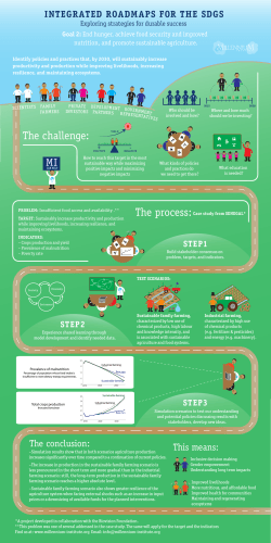


© Copyright 2026