1. business and industrial
2. construction

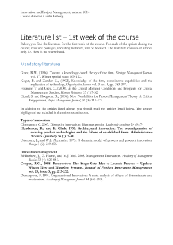
USING LIFE CYCLE COSTING FOR PRODUCT
MANAGEMENT
Jan Vlachý *
Received: 7. 3. 2014
Accepted: 31. 5. 2014
Case study
UDC 658.62
Introducing a case study on product management, this paper applies the Life Cycle
Cost (LCC) method to solve a particular problem of design selection in the area of
mechanical engineering. It is clearly explained and illustrated that various cost
types need to be taken into account, ranging over the whole life of the product
from concept to end-of-life, and related to an appropriate unit of utility. In order
to achieve maximum effect, such a comprehensive economic analysis should
ideally be undertaken at a very early stage of the product’s life cycle, such as its
design or even conception. Advanced techniques, including sensitivity analyses
and simulations, will typically be required to gain an adequate insight into various
processes and uncertainties contained in any realistic life cycle model.
1. INTRODUCTION
As most users of durable goods ultimately find out, a product developed or
purchased at the lowest initial cost need not necessarily be the one which also
provides the same utility at the lowest overall cost. Taken in the broader context
of economic decision-making, product ownership costs, over the whole product
lifecycle, are often significant, sometimes exceeding their acquisition costs by a
multiple. Researchers also argue that up to 70-90 % of these total life cycle
costs become defined already in the design phase (Woodward, 1997; Lindholm
and Suomala, 2004; Bescherer, 2005).
This is the essential reasoning, which has led to the development of the
Life Cycle Costing (LCC) method, originally designed for procurement
*
Jan Vlachy, Senior Researcher, Czech Technical University in Prague, Faculty of Mechanical
Engineering, Karlovo nám. 13, 121 35 Prague 2, Czech Republic. Tel.: +420 224 355 798,
E-mail: [email protected], [email protected]
205
Management, Vol. 19, 2014, 2, pp. 205-218
J. Vlachy: Using life cycle costing for product management
purposes in the U.S. Department of Defense and still used most commonly in
the military sector. The construction industry has since become another major
applicant of LCC, because buildings are typically used and operated over a long
period of time. As a rule of thumb, after six to eight years the operational costs
of a building are as high as the cost of its construction (Woodward, 1997; Staudt
et al., 1999; Opuku, 2013).
A third major promoter of LCC is the public sector, whose heavy
involvement in the area of life cycle cost calculations frequently combines with
Life Cycle Assessment (LCA) studies, focusing primarily on sustainability and
environmental issues. Initial investment costs are still most often used as the
primary or sole criteria in purchase or acquisition decisions. In spite of the
obvious long-term benefits of LCC, its adoption has been relatively slow in
other industries. Applications and analytical approaches are also rather diverse
(Woodward, 1997; Norris, 2001; Lindholm and Suomala, 2004; Dhillon, 2010).
To quote just a few examples, partially related to this paper’s focus, Jun
and Kim (2007) have showed the application of this technique in cost modeling
of the brake module of a train vehicle. Several scenarios have been since with
reduced or increased man hour requirements. Li et al. (2013) described a
framework for the strategic planning of railway maintenance and renewal
projects. Ficko et al. (2005) focused on the total costs of tool manufacture.
Lamb (1996) attempted to connect business performance and competitiveness to
maintenance in the context of paper and pulp industry. He discussed the concept
of availability as a measure of business performance and made reliability and
maintenance operations the key drivers for paper mill performance. Azzopardi
et al. (2011) used LCC to compare the effects of technological advance in
materials development.
This paper strives to summarize the specific features and benefits of life
cycle cost analysis in the particular context of strategic product management. A
case study illustrates the essential points.
2. LCC PRINCIPLES AND IMPLEMENTATION
The fundamental difference between the LCC and conventional
management accounting systems is the tracking and accumulation of costs and
revenues attributable to the product over its full life cycle, which may last for
many years. The life cycle costs of products then comprise all costs attributable
to a product from its conception and pre-production stage to those that
customers incur throughout the life of the product, including the costs of
206
Management, Vol. 19, 2014, 2, pp. 205-218
J. Vlachy: Using life cycle costing for product management
installation, operation, support, maintenance and disposal (Fabrycky and
Blanchard, 1991; Artto, 1994). LCC also typically extends the scope of
applicable costs, included in its analysis (Table 1).
Whereas conventional costing is essentially based on Cost Types I and II
(direct and indirect), LCC usually adds Type III (contingencies), often Type IV
(intangibles), and sometimes (primarily within the domain of public sector
procurement) aspires to involve Type V (externalities) (Norris, 2001; Drury,
2007).
Table 1. Cost type breakdown
Cost Type
Type I:
Direct
Type II:
Indirect
Type III:
Contingent
Type IV:
Intangible
Type V:
External
Description
Direct costs of capital investment, labor, raw material, waste
disposal. May include both recurring and non-recurring costs.
Indirect costs not allocated to the product or process (overhead).
May include both recurring and non-recurring costs.
Contingent costs such as fines and penalties, personal injury or
property damage liabilities, production or service disruption,
competition response etc.
Difficult to measure costs, including consumer acceptance, customer
loyalty, worker morale, community relations, corporate image.
Costs borne by other parties than those directly involved in the life
cycle (e.g. society).
Source: Adapted from Norris (2001), Kong and Frangopol (2003).
There are numerous distinct inputs to a typical LCC model, including, for
instance in the case of engineering products: warranty coverage period, average
material cost of a failure, cost of training, cost of installation, system’s or item’s
listed price, cost of carrying spares in inventory, mean time between failures,
mean time to repair, spares’ requirements, cost of labor per corrective
maintenance action, testing and integration costs, documentation and
compliance costs, as well as time spent for travel (Boussabaine and Kirkham,
2004; Dhillon, 2010).
Clearly, the viability of any LCC analysis ultimately hinges on the
availability of information spanning diverse locations and activities, frequently
not held or collected by the particular decision-making entity. This necessitates
an extensive, and sometimes creative, use of various cost-estimation models,
often including advanced statistical tools. Generally, they may be systematized
into three categories as shown in Table 2.
207
Management, Vol. 19, 2014, 2, pp. 205-218
J. Vlachy: Using life cycle costing for product management
Table 2. Cost estimation model categories
Method
Analogous
Bottom-up
Top-down
(Parametric)
Description
Compares costs according to similarities and differences with other
projects.
Collects all product cost values that are available, making it a
highly data intensive method. Uses e.g. activity based costing.
Derives cost estimating relationships and associated mathematical
algorithms to reach cost estimates. Uses e.g. regression analysis,
fuzzy logic, neural networks.
Source: Adapted from Asiedu and Gu (1998), Boussabaine and Kirkham (2004).
An LCC analysis would often be used when variant solutions of a
particular problem exist, with regards to, for example, design or constructional
alternatives, operational scenarios, logistics, distribution or recycling. In such
cases, relative, rather than absolute, valuation would be required, resulting in
somewhat reduced data requirements (Dhillon, 2010).
Whenever qualitative aspects influence the end-user’s decision, it is
convenient to benchmark LCC analysis against a functional unit, rather than a
particular product or service. This allows a full life cycle comparison of
fundamentally different solutions to the same utility need, which would be
satisfied by a service or a product. Such a functional unit might relate to e.g.
servicing capacity, degree of protection or system performance (Norris, 2001).
From the product’s perspective, the life cycle is divided into several
(usually 3 – 4) phases. The greatest overall effect will typically be achieved by
LCC implementation in the earliest stages of the life cycle, i.e. design and
development. Normally, time value is subsumed in the calculations through
discounting all costs relative to the point of service initiation (Fabrycky and
Blanchard, 1991; Bescherer, 2005; Kapp and Girmscheid, 2005).
3. CASE STUDY
3.1. Problem description
The producer is currently taking a strategic decision, selecting from two
design proposals for a new gear unit to be used in public transport vehicles
(buses). The designs vary in concept; one (A) being an automatic (selfchanging) gearbox, the other one (M) mechanical (manual). The selection
precedes a substantial investment into final product development, certification
208
Management, Vol. 19, 2014, 2, pp. 205-218
J. Vlachy: Using life cycle costing for product management
and pre-production, necessary to construct and deliver trial units to the bus
producer, who has an outstanding tender requirement for replacement vehicles
submitted by the municipal transportation board. Of principal joint concern for
all the parties are total life cycle costs, as these will ultimately be shared
amongst them, albeit indirectly, through tender prices.
Based on thorough research, the gear unit producer has identified three
relevant phases of the life cycle, distinguished by the particular entity retaining
the product. These include the gear unit production (P), its installation into the
bus (N), and its usage in municipal transport (U). Within the life cycle, each
solution (design) features distinct properties, impacting total costs. From the
sole perspective of its production costs, the automatic gear unit is more
expensive, with direct and allocated overhead costs amounting to € 4,800, while
those of the mechanical unit total only € 4,000. Its installation into the vehicle is
also more costly, at € 500, specifically requiring each bus to be initially fitted
with electronic components worth € 700; installation of the mechanical gear
costs just € 400. However, in the phase of use (service), the automatic gear
brings certain benefits. In particular, it reduces average fuel consumption by 0.5
liters per 100 km. It is also expected to lessen the skills requirements for
drivers, and thus staff costs, by € 0.25 per hour.
The mechanical unit has a projected working life of 200,000 km, and will
thereafter be disposed of at a cost of € 500. The automatic unit, whose disposal
cost is also € 500, has a shorter serviceable life of 175,000 km, with a higher
probability of its pre-mature break-down than that of the mechanical gear,
which is much more reliable. However, the automatic gear can be refurbished
by the producer, normally up to two times each, at a cost of € 1,600. An
unscheduled service disruption is estimated to cost € 650 (including opportunity
costs). On average, each vehicle (bus) operates 4,800 hours / year and, over that
time, covers a distance of 180,000 km. The economic life of a bus is 1 million
kilometers (this implies a replacement interval of cca. 5.5 years). The time
factor of production and installation is included in their respective costs, an
annual discount rate of 9% (using continuous compounding) will be used for the
life-cycle stage of product use. Annual deliveries are expected to reach
approximately 50 units.
3.2. Problem solution
While using the LCC method, it is essential to identify all relevant cost
types, and, wherever comparison is undertaken, also to determine an appropriate
209
Management, Vol. 19, 2014, 2, pp. 205-218
J. Vlachy: Using life cycle costing for product management
functional unit, against which total costs will be benchmarked. Several cost
types are involved in this particular case:
• Type I (direct) costs, numerous;
• Type II (indirect) costs are relevant primarily in the production stage,
but many would be essentially equal for both alternatives and therefore
need not be accounted for because the projects are mutually exclusive;
• Type III (contingent) costs relate to the reliability of product A;
• Type IV (intangible) costs may relate e.g. to the acceptance of the
product by the users (i.e. drivers).
Under certain circumstances, Type V costs might also be considered, e.g.
relating to the environmental perspective. In the present case, both variants are,
for the most part, comparable from that point of view. Some differences may
ensue from combustion efficiency (A consuming less fuel) and recycling
(A allowing refurbishment). These are, however, already taken into account
within the frame of other cost types. It is generally assumed that all regulatory
requirements are met and will continue to be so in the foreseeable future.
The life cycle and functional unit costs for product M, all of whose costs
are given as Type I, are quite straightforward to estimate. Its life cycle is
projected to last 200,000 km and includes the costs of production of the gearbox (€ 4,000) and its installation costs (€ 400) at the beginning of the period,
and disposal costs (€ 500) at the end of the period, as shown by Figure 1.
Figure 1. Life cycle time line (unit M)
Source: Author.
There are also costs of operation to consider (staff and fuel), but as these
are only compared on an incremental basis with product A, they will be dealt
with later. Five mechanical gear-box life cycles also exactly fit into the full life
cycle of a bus, which thus becomes irrelevant (if that were not the case, one
210
Management, Vol. 19, 2014, 2, pp. 205-218
J. Vlachy: Using life cycle costing for product management
might have to consider either a premature life cycle termination or extension of
the final gear-box installed in a vehicle before its retirement, as will be shown
later with variant A).
As the two alternatives are not equal in terms of utility per product, having
a different duration and structure of their life cycles, we have to benchmark total
costs against a common functional unit. In the present case, it is most practical
to relate the functional unit to the number of kilometers of service, and we shall
thus select 100,000 kilometers (the actual number being arbitrary).
Using this particular functional unit, it will be effective to relate the
discount rate to the period of 100,000 km, which essentially serves as a measure
of service time. Knowing the annual mileage of a bus (180,000 km), we shall
thus henceforth be using the discount rate of 9% × 100 000 / 180 000 = 5% (per
100 000 km, i.e. 0.56 years). The discounted life cycle cost for the mechanical
gear (excluding costs of operations) can then be calculated as LCM = 4 400 +
500 e-2×5% = € 4,852 (financial formulas using continuous compounding and
their derivations are described in detail by e.g. Los, 2001).
To convert the life cycle cost, which relates to 200,000 kilometers of
service, to the functional unit cost (per 100,000 km of service), we use the
equivalent annual annuity method, deriving the cost per functional unit CM =
4 852 × 5% / (1 – e-2×5%) = € 2 550.
While the Type I and II costs are being assessed deterministically (i.e.
using their best estimate), a fundamentally different approach has to be used
with Type III costs, which constitute statistically random processes. This makes
the cost of the automatic gear unit much more complicated and requires the
creation of a statistical model.
The reliability-based process of unit break-down (for A) will be described
using the simple exponential distribution (Mun, 2006, p. 119) with a mean µ =
300,000 km. Each life cycle of a gear unit is thus going to differ (not only
because of its absolute length, but also the frequency of refits, as well as their
planned or unplanned nature) and there is also due to be a different fit within the
life cycle of the bus. We must now therefore consider the complete life cycle of
the bus, i.e. 1,000,000 km. The unit’s lifecycle will then be determined by a
dynamic process, illustrated by Figure 2, with its control parameters
summarized by Table 3.
211
Management, Vol. 19, 2014, 2, pp. 205-218
J. Vlachy: Using life cycle costing for product management
Figure 2. Life cycle algorithm (unit A)
Source: Author’s algorithm.
Note that a special rule had to be established, in line with operating
manuals and applicable regulations, to mitigate the occurrence of brand new
gear-box installations into vehicles just before their retirement, which would
212
Management, Vol. 19, 2014, 2, pp. 205-218
J. Vlachy: Using life cycle costing for product management
clearly be highly inefficient. This goal has been achieved by stipulating that
refitted gears from retired buses would be used whenever a bus had less than
100,000 km to retirement. The cost differential for fuel ∆F depends on its price p
(per liter) and the consumption differential ∆C described by ∆F = ∆C × p ×
100 000 / 100; the cost differential for staff ∆S depends on the wage differential
∆W as in ∆S = ∆W × 4 800 × 100,000 / 180,000 (each per the functional unit of
100,000 km).
Table 3. Control parameters of the life cycle algorithm (unit A)
Par.
PC
PR
NC
NE
US
UD
λ
ρ
β
ξ
k
m
n
Description
Cost of production (€)
Cost of refurbishment (€)
Cost of installation (€)
Cost of electronics (€)
Cost of service disruption (€)
Cost of disposal (€)
Construction life of gear unit (km)
Actual life of gear unit (km)
Construction life of bus (km)
Maximum life of bus to qualify for new gear-box (km)
Kilometers of service
Maximum number of refits
Number of refits
Spec.
4,800
1,600
500
700
650
500
175,000
stoch.
1,000,000
900,000
var.
2
var.
Source: Author.
The life cycle cost for the automatic gear will be determined using
parametric (Monte Carlo) simulation (Mun, 2006). As we are only concerned
about the differential costs per functional unit, the costs of the mechanical gear,
as well as differential operational costs, will be directly subtracted using a
criteria measure denoted as NAA (Net Advantage of the Automatic gear per
functional unit) and calculated according to:
NAA = CM – LCA × 5% / (1 – e-10×5%) + ∆F + ∆S
(1),
where LCA represents the simulated discounted life cycle cost of the automatic
gear (per its 1 million km life cycle), the term CA = LCA × 5% / (1 – e-10×5%)
stipulating its cost per functional unit (100 000 km), presuming a life cycle
spanning 10 functional units and a discount rate of 5%.
213
Management, Vol. 19, 2014, 2, pp. 205-218
J. Vlachy: Using life cycle costing for product management
Postulating the parameters p = 1.40 € / l, ∆C = 0.50 l / 100 km, and ∆W =
0.25 € / h and assuming batches of 50 units, the simulation output (using 10,000
simulation runs), in line with the annual demand projection, generates an NAA
probability distribution, illustrated by Figure 3. According to its shape and
position, there is a clear advantage to using the automatic gear (with a mean
NAA of € 580 per 100,000 km of use and a negligible probability of attaining a
negative value).
NAA [€ / 100,000 km]
Figure 3. Net Advantage to using Automatic gear unit (base assumptions)
Source: Author’s calculation.
3.3. Sensitivity analysis
Based on the previous result only, it might seem that the automatic gear
should be the obviously preferred choice. There are, however, a number of
underlying assumptions, whose uncertainty has to be properly dealt with. This
process is always an essential component of LCC and uses various kinds of
sensitivity analyses and scenario-based simulations. Accordingly, we shall now
present a rudimentary example of such an approach.
In the present case, crucial uncertainties may be presumed to relate mainly
to the operating cost differential estimates. On the one hand, there is the market
price of fuel factor, which is difficult to predict and volatile over time. Its rising
price increases the NAA, with a positive sensitivity ∆NAA / ∆p = 500 (i.e. an
increase in the oil price by € 1 increases NAA by € 500 per 100,000 km); even
more telling is its break-even point, amounting to just € 0.20 per liter (both of
214
Management, Vol. 19, 2014, 2, pp. 205-218
J. Vlachy: Using life cycle costing for product management
these values can either be inferred analytically, through derivation of (1), or
numerically, using the simulation model). On a stand-alone basis, price risk
would thus be essentially irrelevant, as far as the product selection is concerned.
On the other hand, however, there is a risk that the projected wage
differential would not be sustainable (for example due to trade union pressure,
or the operational necessity to maintain uniform qualification standards for all
drivers). This is essentially a Type IV cost, not to be underrated (more so that it
comes under the auspices of the municipality, not the producer). Based on a
repeated simulation instating ∆W = 0, we find that the resulting NAA distribution
now has a mean of € 0 (standard deviation € 160, assuming the 50 unit batches),
all of a sudden making the fuel price (and possibly other assumptions) an
essential value driver with a dominant influence on the ultimate decision.
Taking such a scenario into account, we would now be inclined to prefer
the automatic gear unit solution only provided fuel prices were projected to rise,
rather than fall in the medium term. This point of view is further facilitated by
the fact that, due to its lower reliability, the automatic gear unit may incur
additional operating risks. For example, an increase in the projected cost of
service disruption (there may be various reasons for such a development,
including regulatory or market-driven) to € 850 (retaining ∆W = 0) results in a
negative mean NAA of – € 70, which would only be mitigated (from the point of
view of the ultimate selection of variant A) by a projected fuel price growth
exceeding € 0.15 per liter.
4. CONCLUSION
In this paper, we have described and shown how the life cycle cost
approach may be of vital assistance for strategic decision-making, such as the
selection of the appropriate product solution. A very high degree of
understanding is obtained, relating to all value-relevant factors and processes
spanning the whole life cycle, and also their particular risks and mutual
relationships. Besides managerial decisions of the individual parties, such as the
designers, producers or users of a product, an LCC analysis may thus also
facilitate their commercial communication or negotiations.
Obviously, as compared to conventional budgeting, the LCC method tends
to involve much more sophisticated tools and procedures, and requires
substantial skills and resources in order to obtain the necessary data.
Outstanding business experience and judgmental skills are also crucial for
achieving a well-substantiated and practicable interpretation of the results of the
215
Management, Vol. 19, 2014, 2, pp. 205-218
J. Vlachy: Using life cycle costing for product management
analysis. Generally, its application may be beneficial wherever significant
investments are being considered, incurring costs, direct or indirect, over
relatively long periods of products’ use. Application of the LCC method, as a
case study for project management, is discussed by the teaching notes,
illustrated by Table 4.
Table 4. Teaching Notes – Instructions on LCC-based project assessment
•
Instructional direction
Introduce the product
life cycle concept
using several practical
examples.
•
•
Introduce and explain
the nature of different
types of costs and
applicable valuation
methods. Highlight
the essence and
importance of using
estimates and
statistical methods in
cost estimation.
Explain the obstacles
and fall-backs when
obtaining data and
assumptions for the
LCC models. Relate
this issue to major
challenges when
interpreting results.
Student understanding
Students focus on the
distinction between
different life cycle
stages and their
respective
contribution to the
total ownership cost.
•
Students should
clearly distinguish
between the cost
types and understand
the basic valuation
methods.
•
•
•
Introduce the concept
of functional unit and
functional unit
costing.
•
•
Explain how various
objectives may be
addressed by different
types of decisionmaker.
•
216
Students should
become comfortable
with collecting and
processing various
types of relevant data
and test hypotheses
using tools like
sensitivity and
scenario analysis.
Students should be
able to design
suitable functional
units and understand
their essential role in
comparative costing.
Students should be
able to identify and
clearly distinguish
between various
utility functions.
•
Discussion or simulation
Identify particular decisionmaking areas where the life
cycle approach makes a
difference compared to the
conventional budgeting
methods.
•
Simulate and discuss the cost
of particular items.
•
Simulate particular models
with a focus on various
sensitivities and
interpretations of results.
Discuss real-life
implications.
•
Using simple cases, propose
appropriate functional units.
How does the functional unit
impact total life cycle cost
results under different
end-users’preferences?
Compare a project‘s total life
cycle cost from a
commercial and a public
entity’s perspective. Discuss
potential conflicts and their
resolution.
•
Management, Vol. 19, 2014, 2, pp. 205-218
J. Vlachy: Using life cycle costing for product management
REFERENCES
1. Artto, K. A. (1994). Life cycle cost concepts and methodologies. Journal of
Cost Management, 8(4),28–32.
2. Azzopardi, B., Emmott, C. J. M., Urbina, A., Krebs, F. C., Mutale, J. &
Nelson, J. (2011). Economic assessment of solar electricity production from
organic-based photovoltaic modules in a domestic environment. Energy &
Environmental Science, 4(10), 3741-3753
3. Asiedu, Y. & Gu, P. (1998). Product life cycle cost analysis: state of the art
review. International Journal of Production Research, 36(4), 883-908.
4. Bescherer, F. (2005). Established life cycle concept in the business
environment. Helsinki: University of Technology.
5. Boussabaine, H. A., & Kirkham, R. J. (2004). Whole life-cycle costing:
risks and risk responses. Oxford: Blackwell Publishing.
6. Dhillon, B. S. (2010). Life cycle costing for engineers. Boca Raton: CRC
Press.
7. Drury, C. (2007). Management and cost accounting. Stamford, Cengage.
8. Fabrycky, W. & Blanchard, B. (1991). Life cycle cost and economic
analysis. New Jersey: Prentice Hall.
9. Ficko, M., Drstvenšek, I., Bresočnik, M., Balič, J. & Vaupotic, B. (2005).
Prediction of total manufacturing cost for stamping on the basis of CADmodel of the finished product. Journal of Materials Processing Technology,
165(1), 1327-1335.
10. Jun, H. K. & Kim, J. H. (2007). Life cycle cost modeling for railway
vehicle. In: Proceedings of International Conference on electrical
Machines and Systems. Seoul, Korea, October 8-11.
11. Kapp, M. J. & Girmscheid, G. (2005). Risk based life cycle cost analysis
model for comparable life cycle project delivery decision taking. In:
Collaboration and Harmonization in Creative Systems. London: Taylor &
Francis, 895-901.
12. Kong, J. S. & Frangopol, D. M. (2003). Life-cycle reliability-based
maintenance cost optimization of deteriorating structures with emphasis on
bridges. Journal of Structural Engineering, 129(6), 818-828.
13. Lamb, R. G. (1996). Determining true cost of maintenance performance can
generate new profits. Pulp & Paper, 70(10), 93-100.
14. Li, R., Landex, A. & Nielsen, O. A. (2013). Framework for railway phasebased planning. In: Trafikdage. Aalborg Universitet, Denmark, August 25 –
26.
15. Lindholm, A. & Suomala, P. (2005). Learning by costing: Sharpening cost
image through life cycle costing? In: The 7th Manufacturing Accounting
Research Conference. Tampere, Finland, May 30 - June 1.
217
Management, Vol. 19, 2014, 2, pp. 205-218
J. Vlachy: Using life cycle costing for product management
16. Los, C. A. (2001). Computational finance: a scientific perspective.
Singapore: World Scientific Publishing.
17. Mun, J. (2006). Modeling risk. Hoboken: John Wiley.
18. Norris, G. A. (2001). Integrating life cycle cost analysis and LCA. The
International Journal of Life Cycle Assessment, 6(2), 118-120.
19. Opoku, A. (2013). The application of whole life costing in the UK
construction industry: benefits and barriers. International Journal of
Architecture, Engineering and Construction, 2(1), 35-42.
20. Staudt, E., Kriegesmann, B. & Thomzig, M. (1999). Facility Management:
Der Kampf um Marktanteile beginnt. Frankfurt: FAZ Verlag.
KORIŠTENJE MODELA IZRAČUNA TROŠKA TIJEKOM ŽIVOTNOG
CIKLUSA U UPRAVLJANJU PROIZVODOM (STUDIJA SLUČAJA)
Sažetak
Koristeći studiju slučaja u upravljanju proizvodom, u ovom se radu primjenjuje metoda
izračuna troškova tijekom cjelokupnog životnog ciklusa proizvoda, kako bi se riješio
specifičan problem izbora dizajna proizvoda u području strojarstva. Pritom se
objašnjava i predočava da u obzir treba uzeti različite vrste troškova, koji se pojavljuju
tijekom cijelog života proizvoda (tj. od njegove konceptualizacije, pa do kraja životnog
ciklusa), a treba ih usporediti s odgovarajućom razinom korisnosti. Da bi se postigao
najveći učinak, ovako bi složenu ekonomsku analizu trebalo obaviti u vrlo ranoj fazi
životnog ciklusa, kao što je faza dizajna ili, čak, inicijalnog osmišljavanja proizvoda.
Pritom će biti potrebno koristiti napredne tehnike, kao što se analiza osjetljivosti i
simulacija, s ciljem odgovarajućeg razumijevanja procesa i neizvjesnosti, koji se
pojavljuju u svim realističnim modelima životnog ciklusa proizvoda.
218