Extended Introduction to Computer Science CS1001.py Lecture 27: Starting to Recap Instructors: Benny Chor, Amir Rubinstein Teaching Assistants: Michal Kleinbort, Yael Baran School of Computer Science Tel-Aviv University Spring Semester, 2013-14 http://tau-cs1001-py.wikidot.com Lecture 27: Plan • Cycles in Linked Lists – An old Debt • A high level view of algorithm, computational problems, and computational complexity. - 2 Algorithmic approaches A crash intro to the P vs. NP problem Map coloring Linked Lists – An old debt Reminder: An alternative to using a contiguous block of memory, is to specify, for each item, the memory location of the next item in the list. We can represent this graphically using a boxes-andpointers diagram: 1 3 2 3 4 Linked Lists Representation (reminder) We introduce two classes. One for each node in the list, and another one to represent a list. The class Node is very simple, just holding two fields, as illustrated in the diagram. class Node (): def __init__ (self, val): self.value = val self.next = None def __repr__ (self): return str(self.value) # return "[" + str(self.value) + "," + str(id(self.next))+ "]" 4 Linked List class (reminder) class Linked_list (): def __init__ (self): self.next = None # using same field name as in Node def __repr__ (self): out = "" p= self.next while (p != None ): out += str(p) + " “ p=p. next return out More methods will be presented in the next slides 5 Perils of Linked Lists With linked lists, we are in charge of memory management, and we may introduce cycles: >>> L = Linked_list() >>> L.next = L >>> L Can we check if a given list includes a cycle? 6 Here we assume a cycle may only occur due to the next pointer pointing to an element that appears closer to the head of the structure. But cycles may occur also due to the “content” field Detecting Cycles: First Variant def detect_cycle1 (lst): dict ={ } p= lst while True : if (p == None ): return False if (p in dict ): return True dict [p] = 1 p = p.next Note that we are adding the whole list element (“box") to the dictionary, and not just its contents. Can we do it more efficiently? In the worst case we may have to traverse the whole list to detect a cycle, so O(n) time in the worst case is inherent. But can we detect cycles using just O(1) additional memory? 7 Detecting cycles: The Tortoise and the Hare Algorithm 8 def detect_cycle2 ( lst ): # The hare moves twice as quickly as the tortoise # Eventually they will both be inside the cycle # and the distance between them will decrease by 1 every # time until they meet. slow = fast = lst while True : if ( slow == None or fast == None ): return if ( fast.next == None ): return slow = slow.next fast = fast.next.next if ( ): return True Detecting cycles: The Tortoise and the Hare Algorithm 9 def detect_cycle2 ( lst ): # The hare moves twice as quickly as the tortoise # Eventually they will both be inside the cycle # and the distance between them will decrease by 1 every # time until they meet. slow = fast = lst while True : if ( slow == None or fast == None ): return False if ( fast.next == None ): The same idea is used in return False Pollard's algorithm for slow = slow.next factoring integers. fast = fast.next.next If interested, take Benny's Intro to modern cryptography if ( slow is fast ): in 2 years return True Testing the cycle detection algorithms The python file contains a function that converts a string to a linked list, and a function that introduces a cycle in a list. >>> lst = string_to_linked_list("abcde") >>> lst a b c d e >>> detect_cycle1(lst) False >>> create_cycle(lst,2,4) >>> detect_cycle1(lst) True >>> detect_cycle2(lst) True 10 Perils of “Regular" Python Lists Even with non-linked lists, mutations may introduce cycles. In this example, either append or assign do the trick. >>> lst =["a","b","c","d","e"] >>> lst.append(lst) >>> lst ['a', 'b', 'c', 'd', 'e', [...]] >>> lst = ["a","b","c","d","e"] >>> lst[3] = lst >>> lst ['a', 'b', 'c', [...] , 'e'] >>> lst[1] = lst >>> lst ['a', [...] , 'c', [...] , 'e'] 11 We see that Python recognizes such cyclical lists and [...] is printed to indicate the fact. Computational Problems and Algorithms • Two central notions in most CS courses • What is a computational problem? • A mapping input  output • What is an algorithm? • • A solution to a computational problem A series of operations that transforms input to output. • What is an operation? • • 12 Context dependent Levels of resolution: • …electron level… • bit level • integer level (add, mult, read, write, compare,…) • data structure level (list sort, matrix mult, tree insert) • …button click in a GUI… Algorithms • In what ways can one describe an algorithm? • • • • • • Code (formal, in some programming language) Pseudo-code: less formal, but avoids the technical details Natural language (Hebrew, Arabic, Russian, Swahili, …) Flow diagram Animation Video… • Implementation of an algorithm • A concrete mechanism capable of executing the algorithm (e.g. code) • Execution of an algorithm • 13 Specific machine(s) at a specific time Algorithmic Approaches • Throughout the course, you have been exposed to several algorithmic approaches. • When facing some computational problem, one should take into consideration these approaches, each with its pros and cons. Or invent a new approach… 14 Iterative Algorithms • Algorithms are not limited to a linear sequence of operations – they usually include control structures. • A basic control structure is the loop (an even more basic one is the conditional – if). • In low level languages (assembly), a loop is implemented with a goto statement. • Most high-level programming languages include while and for loops. • 15 In Python, for loops are somewhat safer, as they are normally used to iterate over finite collections. This is not the case in all languages Complexity • A important measure for an algorithm's efficiency • Time complexity • • number of operations / concrete time measurement as a function of the input size • Space complexity • • maximal number of memory cells allocated simultaneously at any specific step of the algorithm as a function of input size • Recall the key difference between time and space: time cannot be reused. c ∙ g(n) • The O(…) notation • • • 16 • a convenient formalization of complexity asymptotic correlates to "rate of growth" • rather than absolute number of operations hides multiplicative constants and negligible additives t(n) n0 t(n) = O(g(n)) Complexity of Iterative Algorithms • Basic iterative patterns (c is some constant independent of n): 1. 2. 3. i=1 while i < n: i = i +1 1. 2. 3. i=1 while i < n: i=i+c 1. 2. 3. i=n while i > 1: i=i-c (c >0) 1. O(logn) 2. 3. i=1 while i < n: i = i *2 1. 2. 3. i=1 while i < n: i = i *c 1. 2. 3. i=n while i > 1: i=i/c (c >1) 1. 2. 3. i=2 while i < n: i=i*i 1. 2. 3. i=2 while i < n: i = i**c 1. 2. 3. i=n while i > 2: i = i**1/c (c >1) O(n) O(???) • Things get more complicated when we have nested loops that are dependent, as we have seen in many occasions throughout the course. 17 Worst / Best Case Complexity • In many cases, for the same size of input, the content of the input itself affects the complexity. • Examples we have seen? Examples in which this is not the case? • Note that this statement is completely illogical: "The best time complexity is when n is very small…" • Often the average complexity is more informative (e.g. when the worst case is rather rare). However analyzing it is usually more complicated, and requires some knowledge on the distribution of inputs. Assuming distribution is uniform: Taverage (n) = ∑ I ∈Input ( n ) T ( I ) Input (n) examples from our course? 18 - hash operation are O(1) on average (not including comparing/hashing elements) - Quicksort runs on average in O(nlogn) (also best case) Recursive Algorithms • Divide – Conquer – Join Solve smaller instances of the problem and join them • Tips: 1. 2. First define the recursion step: think about only 1 level of the recursion. Then adjust the appropriate base conditions If subproblems repeat, consider memoization to speedup solution • Recursive algorithms seen in our course: Lectures: - Fibonacci, n!, binary search (also seen iterative), Quicksort, Mergesort, Hanoi, 8 queens, … Recitations: - Binom, the "change" problem, maximum (several versions), … HW: - tree stuff (heavyPath, mirror), munch (ahhm, chomp), … 19 Recursion Trees • A useful tool for understanding and analyzing recursion. Recall the Fibonacci recursion tree analysis: O(n/2) O(n) Each node requires O(1) time. = c(1+2+...+2n-1) = c(2n-1) = O(2n) 20 = c(1+2+...+2(n/2)-1) = c(2n/2-1) = O(2n/2) = O(√2n) Recurrence Relations • Another, more compact and formal description of recursive processes is recurrence relations. • Recall the formula for Quicksort's best case t(n) = 2t(n/2) + O(n) • This allows easy categorization of the recursive "pattern": • • • 21 how many recursive calls? of what size each? how much time beyond recursion (for the divide and join stages) Recursive Formulae Summary 𝜑= 22 T(N)=1+T(N-1) ‫קריאות‬ ‫רקורסיביות‬ N-1 ‫פעולות מעבר‬ ‫לרקורסיה‬ 1 ‫ עצרת‬,max1 O(log N) T(N)=1+T(N/2) N/2 1 ‫חיפוש בינרי‬ O(N2) T(N)=N+ T(N-1) N-1 N O(N log N) T(N)=N+2T(N/2) N/2 ,N/2 N Quicksort (worst case) max11 Mergesort Quicksort (best case) max22 O(N) T(N)=N+T(N/2) N/2 O(N) T(N)=1+2T(N/2) N/2 ,N/2 1 max2 O(2N) T(N)=1+2T(N-1) N-1, N-1 1 ‫האנוי‬ T(N)=1+T(N-1)+T(N-2) N-1, N-2 1 ‫פיבונאצ'י‬ 1+ 5 2 ‫סיבוכיות‬ ‫נוסחת נסיגה‬ O(N) O(𝜑N) ‫דוגמא‬ N slicing ‫חיפוש בינארי עם‬ Randomized Algorithms • Apply a random choice at some stage (as opposed to deterministic algorithms). • Also termed probabilistic / coin flipping algorithms • Randomness in this course? - Probabilistic primality testing (with Fermat's little theorem) - Diffie-Hellman protocol for generating a secret shared key over a public communication network - Quicksort (with random pivot selection) - Karp Rabin - Π approximation • What is randomness good for? • • • • 23 Running time improvement (e.g. primality testing) Crypto – secrecy (e.g. DH) Defense against evil opponent / bad luck (e.g. QS, KR) Sampling (e.g. Π) Greedy Algorithms • Do what's best now! Do not look at the larger "picture" • The simple version of Ziv-Lempel compression that we have learned is greedy. • HW7: is this justified in terms of compression efficiency? • Huffman tree construction is also greedy. • Greediness does not necessarily pay off (computationally speaking) 24 image from Wikipedia "Brute Force" Algorithms • Brute force, or exhaustive algorithms, simply "try out" all possible solutions. • When the number of possible solutions is exponential, we do our best to avoid such algorithms. • A short detour: HW6's puzzle problem 25 HW6's puzzle problem • Brute force solution: check all m2! arrangements. • a terrible solution for even relatively small m • Here is a high level description of a possible solution, assuming the puzzle is unique* : 1. find e.g. top-left corner 2. extend it step by step to complete leftmost column 3. extend each leftish cell to a whole row • Not assuming the puzzle is unique, we may consider these approaches: - approach 1: reduce the probability for a wrong stich (but still prob>0, i.e. solution may fail): - By checking more than 1 border before each stich. For example, fill upper row and leftmost column first, then fill up the lines by checking "corners" (see solution sketch in the next slides) - By trying several starting positions - Approach 2: use recursion to examine all possible routes (ensures success) - reminds a bit of the 8 queen problem • Can use hash (of borders) for speedup 26 * each piece has a single neighbor from each side, except the borders that lack some of them HW6's puzzle problem – Solution Sketch def find_right_nbr(piece, puzzle): '''find a neighbor on the right of piece''' for i in range(m): for j in range(m): if right_nbr(piece, puzzle[i][j]): return i,j return None def right_nbr(piece1, piece2): ... def find_down_nbr(piece, puzzle): ... def down_nbr(piece1, piece2): ... def find_top_left(puzzle): for i in range(m): for j in range(m): if is_top_left(puzzle,i,j) == True: return i,j def is_top_left(puzzle,i,j): ... 27 HW6's puzzle problem – Solution Sketch (2) print("Solving puzzle...") result = [[0]*m for i in range(m)] print("Locating top left corner...") i,j = find_top_left(puzzle) result[0][0] = puzzle[i][j] print("Recreating leftmost column...") for i in range(m-1): current = result[i][0] x,y = find_down_nbr(current, puzzle) result[i+1][0] = puzzle[x][y] print("Recreating upper row...") ... print("Recreating rest of puzzle...") for i in range(1,m): for j in range(1,m): x,y = ... result[i][j] = puzzle[x][y] 28 Parallel / Distributed Algorithms • Parallel – if 2 subtasks are independent, solve them at the same time by 2 computers • Distributed – several computing units interact with each other, but there is no high level "manager". In parallel computing there is a central computing unit that acts as the "manager" of the whole process 29 Dictatorship Democracy ‫הצצה אל העולם האפל של הסיבוכיות החישוביות‬ ‫‪NPC‬‬ ‫‪NP‬‬ ‫‪P‬‬ ‫‪30‬‬ ‫קושי של בעיות‬ ‫נבחין בין מצבי הידע הבאים בנוגע לפתרון לבעיות חישוביות‪:‬‬ ‫‪ .1‬בעיות טריוויאליות ‪ -‬בעיות שאנו פשוט יודעים את הפתרון שלהן‪ ,‬מצריכות רק‬ ‫שליפה מהזיכרון *‬ ‫דוגמה‪ :‬כמה זה ‪? 1+2‬‬ ‫‪ .2‬בעיות קלות – איננו יודעים פתרון‪ ,‬אבל יש לנו דרך יעילה** לחשב פתרון‬ ‫דוגמה‪ :‬כמה זה ‪?26-17‬‬ ‫דוגמה‪ :‬כמה פעמים מופיע המילה "‪ "and‬בעמוד הראשי של הניו‪-‬יורק טיימס?‬ ‫דוגמה‪ :‬מיון רשימה‬ ‫‪ .3‬בעיות קשות – לא ידועה ‪ /‬לא קיימת דרך פתרון יעילה‬ ‫)ידועה רק דרך אקספוננציאלית(‬ ‫דוגמה‪ :‬הדפסת כל המעברים בבעיית מגדלי האנוי עבור ‪ n‬דיסקיות‬ ‫‪31‬‬ ‫* מבחינת המחשב‪ ,‬אין באמת בעיות טריוויאלית‪ :‬כל דבר דורש חישוב‪ .‬אבל אם הפתרון שמור‬ ‫איפשהו והמחשב רק שולף אותו‪ ,‬נתייחס לזה כאל בעייה טריוויאלית‪.‬‬ ‫** דרך יעילה = אלגוריתם בזמן ריצה פולינומי‬ ‫מצבי ידע ולמידה‬ ‫אחת ההגדרות של למידה היא מעבר ממצב ידע אחד למצב ידע גבוה יותר‪.‬‬ ‫? = ‪7*8‬‬ ‫בעיות קשות‬ ‫‪32‬‬ ‫בעיות קלות‬ ‫בעיות טריוויאליות‬ ‫בעיה קשה אך קלה לאימות‬ ‫מחלקת הבעיות הקשות מכילה בעיות שלא ידוע להם פתרון פולינומי‪.‬‬ ‫חלק מבעיות אלו מקיימות תכונה מעניינת‪:‬‬ ‫אם נקבל לידנו פתרון חוקי‪ ,‬יש לנו דרך יעילה* לאמת )‪ (verify‬אותו‪.‬‬ ‫דוגמה שראינו בקורס?‬ ‫בעיית הלוגריתם הדיסקרטי )‪.(Discrete Log‬‬ ‫‪ Eve‬לא יודעת איך למצוא את ‪ a‬מתוך ‪.p, g, ga % p‬‬ ‫אבל אם תנסה את כל האפשרויות ו"תיפול" על ‪ a‬מתאים‪,‬‬ ‫היא תוכל לאמת זאת בקלות )כי ‪ Modular exponentiation‬קלה(‪.‬‬ ‫מעתה המונח בעיות קשות יתייחס לסוג זה של בעיות‪,‬‬ ‫ואילו המונח בעיות קשות באמת יתייחס לאלו שידוע שאין להם פתרון פולינומי‪.‬‬ ‫‪33‬‬ ‫* כרגיל‪ ,‬יעיל = בזמן פולינומי‬ ‫‪ 4‬דרגות קושי של בעיות‬ ‫‪ .1‬בעיות טריוויאליות – אנו יודעים את הפתרון שלהן‪ ,‬מצריכות שליפה מהזיכרון‬ ‫‪ .2‬בעיות קלות – איננו יודעים פתרון‪ ,‬אבל יש לנו דרך פולינומית לחשב פתרון‬ ‫דוגמה‪ :‬מיון רשימה‬ ‫‪ .3‬בעיות קשות – איננו יודעים פתרון או דרך יעילה לחשב פתרון‪ ,‬אבל אם נקבל‬ ‫לידנו פתרון חוקי‪ ,‬יש לנו דרך יעילה לאמת אותו‬ ‫דוגמה‪ :‬לוג דיסקרטי‬ ‫‪ .4‬בעיות קשות באמת – קיימות רק דרכים בלתי‪-‬יעילות )אקספוננציאליות(‬ ‫לחישוב פתרון‪.‬‬ ‫דוגמה‪ :‬האנוי‬ ‫‪34‬‬ ‫עוד דוגמה‬ ‫?=‪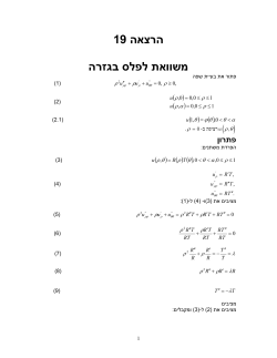x‬‬ ‫‪x7 + 2x4 - 7x + 4 = 0‬‬ ‫בעיה קשה‬ ‫‪35‬‬ ‫‪x2 + 2x - 7 = 0‬‬ ‫בעיה קלה‬ ‫‪x = 1+2‬‬ ‫בעיה טריוויאלית‬ ‫התמודדות חישובית עם בעיות‬ ‫‪ .1‬בעיות טריוויאליות אינן מעניינות מבחינה חישובית‪.‬‬ ‫אלו היו במוקד‬ ‫הקורס שלנו‬ ‫‪ .2‬לבעיות קלות יש אלגוריתמים יעילים‪ ,‬ולכן חישובית אינן צריכות להדאיג‪.‬‬ ‫אבל אפשר לנסות לשפר את האלגוריתמים ‪ /‬להוכיח חסם תחתון לבעיה המעיד‬ ‫כי לא ניתן לשפר עוד‪.‬‬ ‫‪ .3‬דרכים להתמודד עם בעיות קשות‪:‬‬ ‫‪36‬‬ ‫גם אלו נמצאות‬ ‫בלב מדעי המחשב‬ ‫‪(a‬‬ ‫ניסוי וטעייה‪ ,‬או בשם אחר חיפוש ממצה )‪ :(exhaustive search‬מעבר שיטתי על כל‬ ‫האפשרויות ובדיקתן אחת אחת‬ ‫‪(b‬‬ ‫קירובים )‪ – (approximations‬פתרון "כמעט" נכון בזמן פולינומי‬ ‫‪(c‬‬ ‫הנחת הנחות שונות המצמצמות את הבעיה לתת‪-‬משפחות אותן קל יותר לפתור‬ ‫‪(d‬‬ ‫למידה ומחקר בנסיון להפכן לבעיות קלות או אפילו טריוויאליות‪.‬‬ ‫‪ .4‬התמודדות עם בעיות קשות באמת‪ :‬דרכים ‪ a‬עד ‪ c‬לעיל‬ ‫בעיות הכרעה‬ ‫•‬ ‫רוב הבעיות שראינו בקורס עד כה ביקשו לחשב תוצאה כלשהי שהיא מספר‪,‬‬ ‫מחרוזת או אובייקט אחר כלשהו‪:‬‬ ‫חיפוש‪ :‬רשימה ואיבר ‪x‬‬ ‫‪ ‬המיקום של ‪ x‬ברשימה‪ ,‬אם קיים‬ ‫לוג דיסקרטי‪p, g, ga % p :‬‬ ‫‪a‬‬ ‫‪...‬‬ ‫•‬ ‫נגביל כעת את הדיון לבעיות הכרעה‪:‬‬ ‫בעיות שמבקשות תשובה "כן" ‪" /‬לא" בלבד לשאלה כלשהי‪.‬‬ ‫רוב הבעיות שאינן בעיות הכרעה ניתנות לניסוח כבעיות הכרעה‪:‬‬ ‫חיפוש‪ :‬רשימה ואיבר ‪x‬‬ ‫‪ ‬האם ‪ x‬ברשימה ?‬ ‫לוג דיסקרטי‪ p, g, ga%p :‬ובנוסף מספר ‪k‬‬ ‫‪37‬‬ ‫‪ ‬האם קיים ‪? a<k‬‬ ‫דוגמה‪ :‬צביעת מפות‬ ‫)מתוך האתר "מדעי המחשב ללא מחשב"‬ ‫‪.(http://csu-il.blogspot.com‬‬ ‫להלן מפה מדינית‪:‬‬ ‫נגדיר צביעה חוקית של מפה‪:‬‬ ‫צביעה של כל מדינה בצבע אחד‪ ,‬כך שאין‬ ‫שתי מדינות גובלות באותו צבע‪.‬‬ ‫שאלות‪:‬‬ ‫‪38‬‬ ‫‪-‬‬ ‫האם ניתן לצבוע את המפה הזו ב‪ 2 -‬צבעים?‬ ‫‪-‬‬ ‫‪ 3‬צבעים?‬ ‫‪-‬‬ ‫‪ 4‬צבעים?‬ ‫‪ 2‬צבעים‬ ‫‪ 3‬צבעים‬ ‫‪ 4‬צבעים‬ ‫‪ 5‬צבעים‬ ‫יש מפה‬ ‫כן‬ ‫‪‬‬ ‫‪‬‬ ‫‪‬‬ ‫כל מפה‬ ‫לא‬ ‫לא‬ ‫???‬ ‫???‬ ‫צביעת מפות – ייצוג והכללה‬ ‫מפה ניתנת לייצוג באמצעות גרף )‪ – (Graph‬אוסף של קדקדים וקשתות‪.‬‬ ‫צמתים = המדינות‬ ‫קשתות = בין שתי מדינות שכנות‬ ‫צביעה =‬ ‫מיפוי מצמתים למספרים …‪1,2,3,‬‬ ‫ננסח את השאלות מהשקף הקודם באופן כללי‪ ,‬וכשאלת הכרעה‪:‬‬ ‫בהינתן גרף ומספר ‪ ,k‬האם ניתן לצבוע את הגרף באמצעות ‪ k‬צבעים בלבד?‬ ‫‪39‬‬ ‫צביעת גרף – ‪ 2‬צבעים‬ ‫תנאי להיותו של גרף ‪-2‬צביע )‪(2-colorable‬‬ ‫גרף ניתן לצביעה ב‪ 2 -‬צבעים אם"ם אין בו מעגלים באורך איזוגי‪.‬‬ ‫גרף כזה מכונה גם גרף דו‪-‬צדדי )‪.(Bipartite‬‬ ‫‪40‬‬ ‫צביעת גרף ב‪ 2-‬צבעים ‪ -‬סיבוכיות‬ ‫שאלה‪ :‬מה דרגת הקושי של הבעיה "האם גרף ניתן לצביעה ב‪ 2 -‬צבעים"?‬ ‫האלגוריתם עובר על כל צומת ועל כל קשת פעם אחת‪.‬‬ ‫אם גודל הקלט הוא מספר הקשתות )‪ (m‬ומספר הצמתים )‪ ,(n‬ניתן להשיג‬ ‫סיבוכיות של )‪ ,O(n+m‬כלומר ליניארית‪.‬‬ ‫לכן בדיקה האם גרף הוא ‪-2‬צביע היא בעיה קלה חישובית‪.‬‬ ‫‪41‬‬ ‫גרף מישורי‬ ‫לפני שנחשוף עוד תוצאה מפורסמת‪ ,‬נשים לב לתכונה הבאה‪:‬‬ ‫גרף שמייצג מפה מישורית ניתן לשרטוט כאשר אף קשת לא חותכת אף קשת‬ ‫אחרת‪.‬‬ ‫גרף כזה נקרא גרף מישורי )‪.(planar graph‬‬ ‫‪42‬‬ ‫‪ 4‬צבעים בגרף מישורי‬ ‫מתי גרף מישורי הוא ‪-4‬צביע )‪? (4-colorable‬‬ ‫תמיד!!‬ ‫משפט ארבעת הצבעים‪ :‬כל גרף מישורי ניתן לצביעה ב‪ 4 -‬צבעים‪.‬‬ ‫בשנת ‪ 1852‬צעיר בריטי בשם פרנסיס גאתרי ניסח זאת כהשערה‪.‬‬ ‫במשך למעלה מ‪ 120 -‬שנה טובי המתמטיקאים בעולם ניסו להוכיח את השערת ארבעת הצבעים ללא הצלחה‪.‬‬ ‫המשפט הוכח בשנת ‪ .1976‬ההוכחה מראה שניתן לסווג כל דוגמה נגדית אפשרית לאחת מ‪ 1936 -‬סוגי מפות‪.‬‬ ‫אחד מצעדי ההוכחה כולל בחינת סוגים אלו באמצעות מחשב‪.‬‬ ‫ההוכחה שנויה במחלוקת מבחינה פילוסופית‪ .‬מדוע? מה דעתכם?‬ ‫שאלה‪ :‬לאיזו קטגוריה שייכת הבעיה "האם גרף מישורי ניתן לצביעה ב‪ 4 -‬צבעים"?‬ ‫תשובה‪ :‬זוהי בעיה טריוויאלית‪.‬‬ ‫‪43‬‬ ‫אבל‪ :‬בעיית מציאת צביעה ב‪ 4 -‬צבעים לגרף מישורי‪ ,‬אם קיימת‪ ,‬איננה כזו‪.‬‬ ‫‪ 3‬צבעים?‬ ‫לא ידוע כיום אלגוריתם יעיל שעונה "כן"‪"/‬לא" לשאלה‪:‬‬ ‫בהינתן גרף כלשהו‪ ,‬האם ניתן לצבוע אותו ב‪ 3 -‬צבעים?‬ ‫כלומר הבעיה איננה קלה‪.‬‬ ‫האם לדעתכם היא קשה או קשה באמת?‬ ‫במילים אחרות‪ :‬אם נתון לנו גרף כלשהו‪ ,‬ונתונה צביעה חוקית שלו ב‪ 3 -‬צבעים האם‬ ‫ניתן לוודא ביעילות שזוהי אכן צביעה חוקית?‬ ‫מסקנה‪ :‬הבעיה "האם גרף כלשהו ניתן לצביעה ב‪ 3 -‬צבעים" היא בעיה קשה‪.‬‬ ‫למעשה‪ ,‬המסקנה נכונה לכל מספר צבעים ‪k>2‬‬ ‫‪44‬‬ ‫)לא עבור המקרה הפרטי של גרף מישורי‪ ,‬כאמור(‪.‬‬ ‫‪P = NP‬‬ ‫?‬ ‫מחלקת בעיות ההכרעה הקלות מסומנת ‪(Polynomial) P‬‬ ‫מחלקת בעיות ההכרעה הקשות מסומנת ‪,Non-deterministic polynomial) NP‬‬ ‫מה היחס בין שתי המחלקות הללו?‬ ‫הסבר ודיון‪.‬‬ ‫‪P=NP‬‬ ‫לא נסביר‪(...‬‬ ‫?‬ ‫‪NP‬‬ ‫‪P‬‬ ‫השאלה הפתוחה הגדולה של מדעי המחשב )הפרס ‪ -‬מיליון דולר במזומן ותהילת עולם(‪:‬‬ ‫האם היכולת לזהות ביעילות פתרון חוקי של בעיה מעידה על יכולת לפתור אותה‬ ‫ביעילות?‬ ‫פורמלית‪ :‬האם ‪?P=NP‬‬ ‫רוב מדעני המחשב סבורים ש‪ .P≠NP -‬יש לכך תימוכין מכיוונים שונים‪,‬‬ ‫אך זה מעולם לא הוכח‪.‬‬ ‫‪45‬‬ ‫בדיקת ראשוניות )‪(Primality testing‬‬ ‫הבעיה‪ :‬בהינתן מספר שלם חיובי ‪ ,N‬האם הוא ראשוני?‬ ‫עד לא מזמן ידעו לומר שהבעיה ב‪.NP -‬‬ ‫ב‪ 2002 -‬נתגלה שהבעיה למעשה ב‪.P -‬‬ ‫הערה‪ :‬יש להבדיל בין בדיקת ראשוניות לבין פירוק לגורמים ראשוניים‪.‬‬ ‫לבעייה אחרונה לא ידוע אלגוריתם פולינומי כיום‪.‬‬ ‫שאלה‪ :‬האם בעיית הפירוק לגורמים ב‪?NP -‬‬ ‫‪46‬‬ ‫המחלקה ‪NPC‬‬ ‫• ‪ NPC‬הוא קיצור של ‪) NP-Complete‬בעברית‪-NP :‬שלם(‪.‬‬ ‫• לא נסביר את השם הזה‪...‬‬ ‫• זוהי תת מחלקה של ‪ NP‬הכוללת למעלה מ‪ 1000 -‬בעיות בעלות התכונה המפתיעה הבאה‪:‬‬ ‫‪ (1‬אם לאחת מהן יש פתרון פולינומי ‪ ‬לכולן יש‬ ‫‪ (2‬אם לאחת מהן אין פתרון פולינומי ‪ ‬לאף אחת אין‬ ‫• ניתן להראות שבמקרה ‪ ,P=NP (1‬ואילו במקרה ‪P ≠ NP (2‬‬ ‫ומכאן העניין הרב שיש במחלקה זו‪.‬‬ ‫‪P=NP=NPC‬‬ ‫?‬ ‫‪NP‬‬ ‫‪NPC‬‬ ‫‪P‬‬ ‫• בעיית צביעה ב‪ 3 -‬צבעים שייכת ל‪.NPC -‬‬ ‫• בעיית הלוג הדיסקרטי שייכת ל‪ ,NP -‬ולא ידוע אם היא שייכת גם ל‪ ,NPC -‬או שאולי ל‪.P -‬‬ ‫‪47‬‬ ‫עוד דוגמה‪ :‬שבעת הגשרים של ‪Königsberg‬‬ ‫• ‪ – Königsberg‬כיום קלינינגרד ברוסיה‬ ‫• בעיה שנוסחה ע"י לאונרד אוילר‪ ,‬ב‪1735 -‬‬ ‫• נחשבת לפרסום הראשון ב"תורת הגרפים" – לימים ענף מרכזי במדעי המחשב‬ ‫• האם ניתן להתחיל מנקודה מסוימת בעיר‪ ,‬לעבור בכל הגשרים בדיוק פעם אחת‪ ,‬ולחזור‬ ‫לאותה נקודה?‬ ‫‪48‬‬ ‫מידול והפשטה )‪(abstraction‬‬ ‫• האם ניתן להתחיל מנקודה מסוימת בעיר‪ ,‬לעבור בכל הגשרים בדיוק פעם אחת‪,‬‬ ‫ולחזור לאותה נקודה?‬ ‫• מה הפרטים החשובים כאן?‬ ‫האם יש בגרף מסלול שעובר בכל‬ ‫קשת בדיוק פעם אחת?‬ ‫‪49‬‬ ‫מסלול ‪ /‬מעגל אוילר‬ ‫• הגדרה‪ :‬מסלול אוילר בגרף הוא מסלול שעובר בכל קשת בדיוק פעם אחת‪.‬‬ ‫אם מסלול אוילר מתחיל ונגמר באותו צומת‪ ,‬הוא ייקרא מעגל אוילר‪.‬‬ ‫• השאלה שלנו אם כן הפכה להיות‪ :‬מתי גרף מכיל מסלול ‪ /‬מעגל אוילר?‬ ‫• משפט )אוילר‪:(1736 ,‬‬ ‫גרף קשיר* מכיל "מסלול אוילר" אם כל צמתיו‪ ,‬למעט בדיוק ‪ ,2‬בעלי דרגה** זוגית‪.‬‬ ‫והוא מכיל "מעגל אוילר" אם כל צמתיו בעלי דרגה זוגית‪.‬‬ ‫* גרף קשיר – מכל צומת ניתן להגיע לכל צומת‬ ‫** דרגה של צומת ‪ -‬כמות הקשתות שנוגעות בצומת‬ ‫‪50‬‬ ‫‪House of Santa‬‬ ‫• האם תוכלו לצייר את הבית מבלי להרים את העיפרון?‬ ‫האם יש בגרף מסלול אוילר?‬ ‫• הפשטה מאפשרת לראות דמיון בין בעיות !‬ ‫‪51‬‬ ‫מסלולי אוילר ‪ /‬המילטון‬ ‫מסלול אוילר )‪ :(Euler‬מסלול שעובר בכל קשתות הגרף בדיוק פעם אחת‪.‬‬ ‫הבעיה "האם גרף קשיר מכיל מסלול אוילר" ניתנת לפתרון בזמן פולינומי‪:‬‬ ‫עוברים על הגרף ובודקים כמה צמתים יש עם דרגה איזוגית‪.‬‬ ‫אם יש ‪ 0‬או ‪ 2‬עונים "כן"‪ ,‬אחרת עונים "לא"‪.‬‬ ‫‪ ‬בעיית מסלול אוילר שייכת למחלקה ‪.P‬‬ ‫מסלול המילטון )‪ :(Hamilton‬מסלול שעובר בכל צמתי הגרף בדיוק פעם אחת‪.‬‬ ‫למרות הדמיון בין הבעיות‪ ,‬לא ידוע כיום אלגוריתם פולינומי לבעיה זו‪.‬‬ ‫שאלה‪ :‬האם הבעייה קשה או קשה באמת?‬ ‫שאלה‪ :‬האם ייתכן שהבעיה בכל זאת ב‪?P -‬‬ ‫‪52‬‬ ‫בעיות קשות עוד יותר ?‬ ‫• האם יש בעיות קשות יותר מהבעיות ה"קשות באמת" ?‬ ‫• האם יש בעיות שבכלל לא ניתן לפתור בזמן סופי ?‬ ‫• בשיעור הבא )והאחרון(‪...‬‬ ‫• כל הנ"ל יילמד לעומק ובאופן פורמלי הרבה יותר בקורס מודלים חישוביים‬ ‫‪53‬‬